2D Robot Localization on Real Data

Goals of this script:

• apply the UKF for the 2D robot localization example on real data.

We assume the reader is already familiar with the considered problem described in the tutorial.

We address the same problem as described in the tutorial on our own data.

Import

from ukfm import LOCALIZATION as MODEL
import ukfm
import numpy as np
import matplotlib
ukfm.utils.set_matplotlib_config()

Model and Data

This script uses the LOCALIZATION() model.

Instead of creating data, we load recorded data. We have recorded five sequences (sequence 2 and 3 are the more interesting).

# sequence number
n_sequence = 3
# GPS frequency (Hz)
gps_freq = 2
# GPS noise standard deviation (m)
gps_std = 0.1
# load data
states, omegas, ys, one_hot_ys, t = MODEL.load(n_sequence, gps_freq, gps_std)

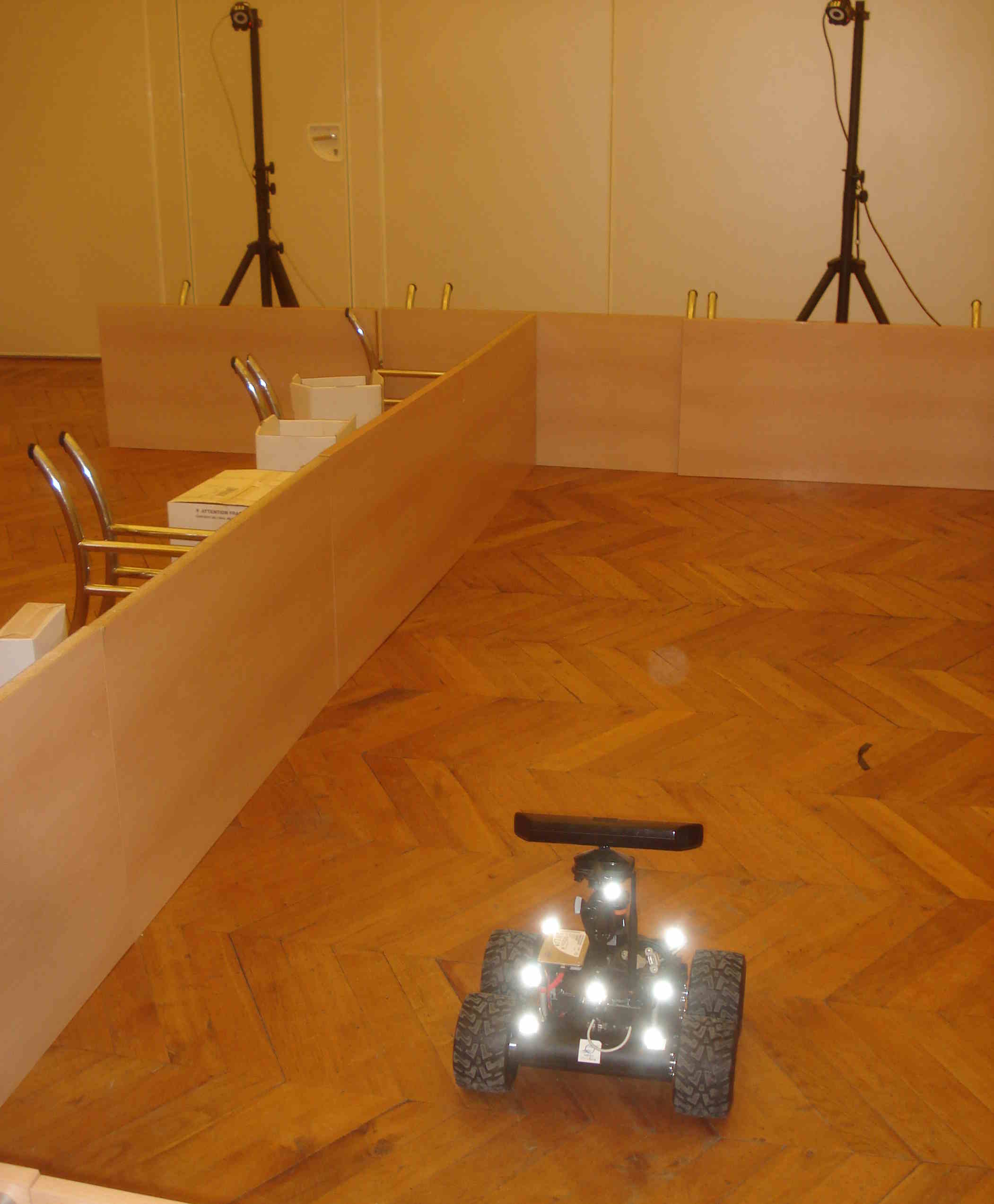
Data has been obtained in an experiment conducted at the Centre for Robotics, MINES ParisTech. We used a so-called Wifibot, which is a small wheeled robot equipped with independent odometers on the left and right wheels, see figure. A set of seven highly precise cameras, the OptiTrack motion capture system, provide the reference trajectory (ground truth) with sub-millimeter precision at a rate of 120 Hz.

Testing arena with Wifibot robot in the foreground of the picture. We can also see two of the seven Optitrack cameras in the background.

We define noise odometry standard deviation for the filter.

odo_std = np.array([0.15,   # longitudinal speed
                    0.05,   # transverse shift speed
                    0.15])  # differential odometry

Filter Design

We embed here the state in \(SE(2)\) with left multiplication, i.e.

• the retraction \(\varphi(.,.)\) is the \(SE(2)\) exponential, where the state multiplies on the left the uncertainty \(\boldsymbol{\xi}\).

• the inverse retraction \(\varphi^{-1}_.(.)\) is the \(SE(2)\) logarithm.

We define the filter parameters based on the model parameters.

# propagation noise covariance matrix
Q = np.diag(odo_std ** 2)
# measurement noise covariance matrix
R = gps_std ** 2 * np.eye(2)
# sigma point parameters
alpha = np.array([1e-3, 1e-3, 1e-3])

Filter Initialization

We initialize the filter with the true state plus an initial heading error of 30°, and set corresponding initial covariance matrices.

# "add" orientation error to the initial state
SO2 = ukfm.SO2
state0 = MODEL.STATE(Rot=states[0].Rot.dot(SO2.exp(30/180*np.pi)),
                     p=states[0].p)
# initial state uncertainty covariance matrix
P0 = np.zeros((3, 3))
# The state is not perfectly initialized
P0[0, 0] = (30/180*np.pi)**2

We define the filter as an instance of the UKF class.

ukf = ukfm.UKF(state0=state0,               # initial state
               P0=P0,                       # initial covariance
               f=MODEL.f,                   # propagation model
               h=MODEL.h,                   # observation model
               Q=Q,                         # process noise covariance
               R=R,                         # observation noise covariance
               phi=MODEL.left_phi,          # retraction function
               phi_inv=MODEL.left_phi_inv,  # inverse retraction function
               alpha=alpha                  # sigma point parameters
               )

Before launching the filter, we set a list for recording estimates along the full trajectory and a 3D array to record covariance estimates.

N = t.shape[0]
ukf_states = [ukf.state]
ukf_Ps = np.zeros((N, 3, 3))
ukf_Ps[0] = ukf.P

Filtering

The UKF proceeds as a standard Kalman filter with a for loop.

# measurement iteration number (first measurement is for n == 0)
k = 1
for n in range(1, N):
    # propagation
    dt = t[n] - t[n-1]
    ukf.propagation(omegas[n-1], dt)
    # update only if a measurement is received
    if one_hot_ys[n] == 1:
        ukf.update(ys[k])
        k += 1
    # save estimates
    ukf_states.append(ukf.state)
    ukf_Ps[n] = ukf.P

Results

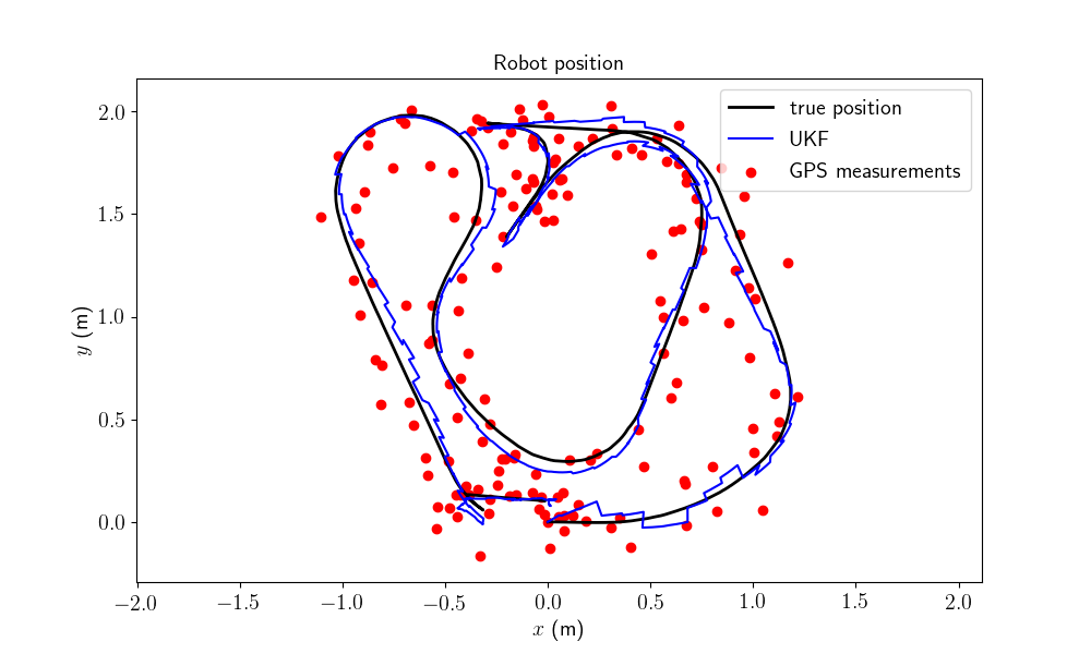
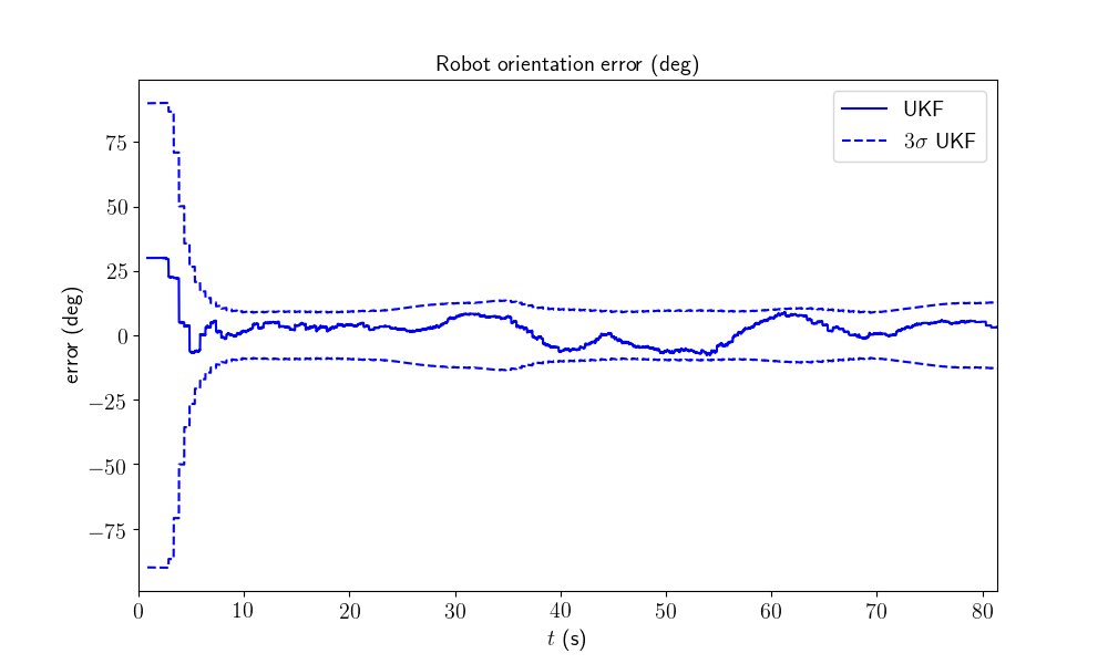
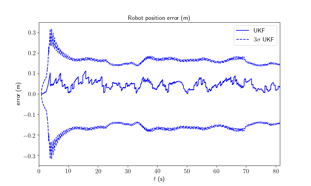
We plot the trajectory, the measurements and the estimated trajectory. We then plot the position and orientation error with 95% (\(3\sigma\)) confident interval.

MODEL.plot_wifibot(ukf_states, ukf_Ps, states, ys, t)

• 
• 
• 

All results are coherent. This is convincing as the initial heading error is relatively high.

Conclusion

This script applies the UKF for localizing a robot on real data. The filter works well on this localization problem on real data, with moderate initial heading error.

You can now:

• test the UKF on different sequences.

• address the UKF for the same problem with range and bearing measurements of known landmarks.