IMU-GNSS Sensor-Fusion on the KITTI Dataset

Goals of this script:

• apply the UKF for estimating the 3D pose, velocity and sensor biases of a vehicle on real data.

• efficiently propagate the filter when one part of the Jacobian is already known.

• efficiently update the system for GNSS position.

We assume the reader is already familiar with the approach described in the tutorial and in the 2D SLAM example.

This script proposes an UKF to estimate the 3D attitude, the velocity, and the position of a rigid body in space from inertial sensors and position measurement.

We use the KITTI data that can be found in the iSAM repo (examples folder).

Import

from scipy.linalg import block_diag
import ukfm
import numpy as np
import matplotlib
ukfm.set_matplotlib_config()

Model and Data

This script uses the IMUGNSS() model that loads the KITTI data from text files. The model is the standard 3D kinematics model based on inertial inputs.

MODEL = ukfm.IMUGNSS
# observation frequency (Hz)
GNSS_freq = 1
# load data
omegas, ys, one_hot_ys, t = MODEL.load(GNSS_freq)
N = t.shape[0]
# IMU noise standard deviation (noise is isotropic)
imu_std = np.array([0.01,     # gyro (rad/s)
                    0.05,     # accelerometer (m/s^2)
                    0.000001, # gyro bias (rad/s^2)
                    0.0001])  # accelerometer bias (m/s^3)
# GNSS noise standard deviation (m)
GNSS_std = 0.05

The state and the input contain the following variables:

states[n].Rot     # 3d orientation (matrix)
states[n].v       # 3d velocity
states[n].p       # 3d position
states[n].b_gyro  # gyro bias
states[n].b_acc   # accelerometer bias
omegas[n].gyro    # vehicle angular velocities
omegas[n].acc     # vehicle specific forces

A measurement ys[k] contains a GNSS (position) measurement.

Filter Design and Initialization

We now design the UKF on parallelizable manifolds. This script embeds the state in \(SO(3) \times \mathbb{R}^{12}\), such that:

• the retraction \(\varphi(.,.)\) is the \(SO(3)\) exponential for orientation, and the vector addition for the remaining part of the state.

• the inverse retraction \(\varphi^{-1}_.(.)\) is the \(SO(3)\) logarithm for orientation and the vector subtraction for the remaining part of the state.

Remaining parameter setting is standard.

# propagation noise covariance matrix
Q = block_diag(imu_std[0]**2*np.eye(3), imu_std[1]**2*np.eye(3),
               imu_std[2]**2*np.eye(3), imu_std[3]**2*np.eye(3))
# measurement noise covariance matrix
R = GNSS_std**2 * np.eye(3)

We use the UKF that is able to infer Jacobian to speed up the update step, see the 2D SLAM example.

# sigma point parameters
alpha = np.array([1e-3, 1e-3, 1e-3, 1e-3, 1e-3])
# for propagation we need the all state
red_idxs = np.arange(15)  # indices corresponding to the full state in P
# for update we need only the state corresponding to the position
up_idxs = np.array([6, 7, 8])

We initialize the state with zeros biases. The initial covariance is non-null as the state is not perfectly known.

# initial uncertainty matrix
P0 = block_diag(0.01*np.eye(3), 1*np.eye(3), 1*np.eye(3),
                0.001*np.eye(3), 0.001*np.eye(3))
# initial state
state0 = MODEL.STATE(
    Rot=np.eye(3),
    v=np.zeros(3),
    p=np.zeros(3),
    b_gyro=np.zeros(3),
    b_acc=np.zeros(3))

As the noise affecting the dynamic of the biases is trivial (it is the identity), we set our UKF with a reduced propagation noise covariance, and manually set the remaining part of the Jacobian.

# create the UKF
ukf = ukfm.JUKF(state0=state0, P0=P0, f=MODEL.f, h=MODEL.h, Q=Q[:6, :6],
                phi=MODEL.phi, alpha=alpha, red_phi=MODEL.phi,
                red_phi_inv=MODEL.phi_inv, red_idxs=red_idxs,
                up_phi=MODEL.up_phi, up_idxs=up_idxs)
# set variables for recording estimates along the full trajectory
ukf_states = [state0]
ukf_Ps = np.zeros((N, 15, 15))
ukf_Ps[0] = P0
# the part of the Jacobian that is already known.
G_const = np.zeros((15, 6))
G_const[9:] = np.eye(6)

Filtering

The UKF proceeds as a standard Kalman filter with a for loop.

# measurement iteration number
k = 1
for n in range(1, N):
    # propagation
    dt = t[n]-t[n-1]
    ukf.state_propagation(omegas[n-1], dt)
    ukf.F_num(omegas[n-1], dt)
    # we assert the reduced noise covariance for computing Jacobian.
    ukf.Q = Q[:6, :6]
    ukf.G_num(omegas[n-1], dt)
    # concatenate Jacobian
    ukf.G = np.hstack((ukf.G, G_const*dt))
    # we assert the full noise covariance for uncertainty propagation.
    ukf.Q = Q
    ukf.cov_propagation()
    # update only if a measurement is received
    if one_hot_ys[n] == 1:
        ukf.update(ys[k], R)
        k = k + 1
    # save estimates
    ukf_states.append(ukf.state)
    ukf_Ps[n] = ukf.P

Results

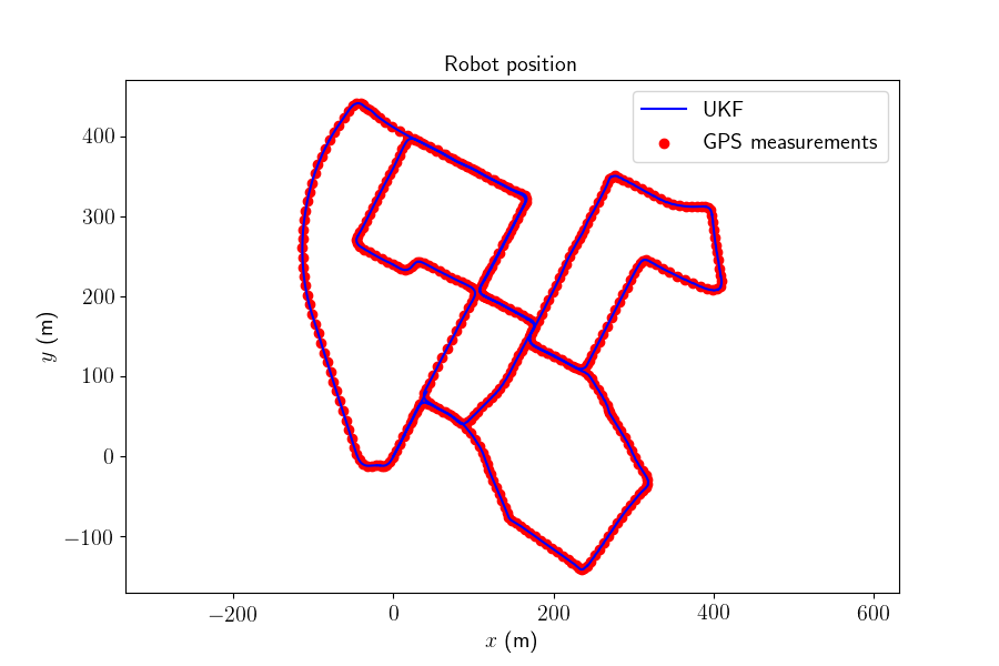
We plot the estimated trajectory.

MODEL.plot_results(ukf_states, ys)

Results are coherent with the GNSS. As the GNSS is used in the filter, it makes no sense to compare the filter outputs to the same measurement.

Conclusion

This script implements an UKF for sensor-fusion of an IMU with GNSS. The UKF is efficiently implemented, as some part of the Jacobian are known and not computed. Results are satisfying.

You can now:

• increase the difficulties of the example by reduced the GNSS frequency or adding noise to position measurements.

• implement the UKF with different uncertainty representations, as viewing the state as an element \(\boldsymbol{\chi} \in SE_2(3) \times \mathbb{R}^6\). We yet provide corresponding retractions and inverse retractions.