Pendulum Example

The set of all points in the Euclidean space \(\mathbb{R}^{3}\), that lie on the surface of the unit ball about the origin belong to the two-sphere manifold,

\[\mathbb{S}^2 = \left\{ \mathbf{x} \in \mathbb{R}^3 \mid \|\mathbf{x}\|_2 = 1 \right\},\]

which is a two-dimensional manifold. Many mechanical systems such as a spherical pendulum, double pendulum, quadrotor with a cable-suspended load, evolve on either \(\mathbb{S}^2\) or products comprising of \(\mathbb{S}^2\).

In this script, we estimate the state of a system living on the sphere but where observations are standard vectors. See the description of the spherical pendulum dynamics in [SE19], Section 7, and [KS19].

Import

from scipy.linalg import block_diag
import ukfm
import numpy as np
import matplotlib
ukfm.utils.set_matplotlib_config()

Model and Simulation

This script uses the PENDULUM() model that requires the sequence time and the model frequency.

# sequence time (s)
T = 10
# model frequency (Hz)
model_freq = 100
# create the model
model = ukfm.PENDULUM(T, model_freq)

The true trajectory is computed along with empty inputs (the model does not require any input) after we define the noise standard deviation affecting the dynamic.

# model noise standard deviation (noise is isotropic)
model_std = np.array([1/180*np.pi,    # orientation (rad)
                      1/180*np.pi])   # orientation velocity (rad/s)
# simulate true states and noisy inputs
states, omegas = model.simu_f(model_std)

The state and the input contain the following variables:

states[n].Rot  # 3d orientation (matrix)
states[n].u    # 3d angular velocity
omegas[n]      # empty input

The model dynamics is based on the Euler equations of pendulum motion.

We compute noisy measurements at low frequency based on the true states.

# observation frequency (Hz)
obs_freq = 20
# observation noise standard deviation (m)
obs_std = 0.02
# simulate landmark measurements
ys, one_hot_ys = model.simu_h(states, obs_freq, obs_std)

We assume observing the position of the state only in the \(yz\)-plan.

Filter Design and Initialization

We embed the state in \(SO(3) \times \mathbb{R} ^3\) with left multiplication, such that:

• the retraction \(\varphi(.,.)\) is the \(SO(3)\) exponential for orientation where the state multiplies the uncertainty on the left, and the vector addition for the velocity.

• the inverse retraction \(\varphi^{-1}_.(.)\) is the \(SO(3)\) logarithm for orientation and the vector subtraction for the velocity.

Remaining parameter setting is standard.

# propagation noise covariance matrix
Q = block_diag(model_std[0]**2*np.eye(3), model_std[1]**2*np.eye(3))
# measurement noise covariance matrix
R = obs_std**2*np.eye(2)
# initial uncertainty matrix
P0 = block_diag((45/180*np.pi)**2*np.eye(3), (10/180*np.pi)**2*np.eye(3))
# sigma point parameters
alpha = np.array([1e-3, 1e-3, 1e-3])
state0 = model.STATE(Rot=np.eye(3), u=np.zeros(3))
ukf = ukfm.UKF(state0=state0, P0=P0, f=model.f, h=model.h, Q=Q, R=R,
               phi=model.phi, phi_inv=model.phi_inv, alpha=alpha)
# set variables for recording estimates along the full trajectory
ukf_states = [state0]
ukf_Ps = np.zeros((model.N, 6, 6))
ukf_Ps[0] = P0

Filtering

The UKF proceeds as a standard Kalman filter with a for loop.

# measurement iteration number
k = 1
for n in range(1, model.N):
    # propagation
    ukf.propagation(omegas[n-1], model.dt)
    # update only if a measurement is received
    if one_hot_ys[n] == 1:
        ukf.update(ys[k])
        k = k + 1
    # save estimates
    ukf_states.append(ukf.state)
    ukf_Ps[n] = ukf.P

Results

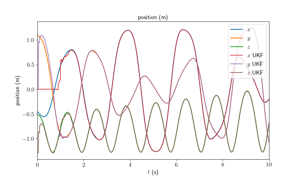
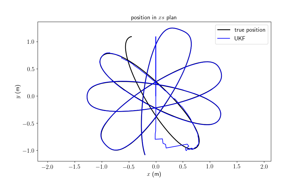
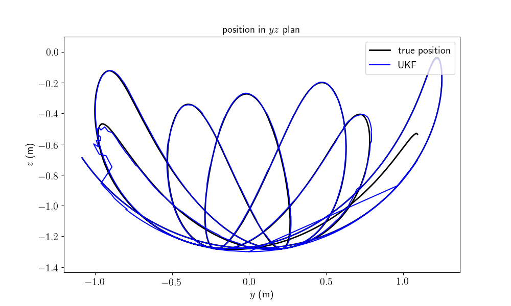
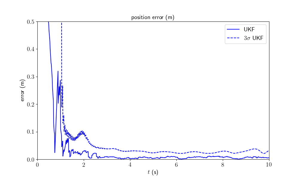
We plot the position of the pendulum as function of time, the position in the \(xy\) plan and the position in the \(yz\) plan (we are more interested in the position of the pendulum than its orientation). We compute the \(3\sigma\) interval confidence by leveraging the covariance retrieval proposed in [BBB19], Section V-B.

model.plot_results(ukf_states, ukf_Ps, states)

• 
• 
• 
• 

On the first plot, we observe that even if the state is unaccurately initialized, the filter estimates the depth position (\(x\) axis) of the pendulum whereas only the \(yz\) position of the pendulum is observed.

The second and third plots show how the filter converges to the true state. Finally, the last plot reveals the consistency of the filter, where the interval confidence encompasses the error.

Conclusion

This script shows how well works the UKF on parallelizable manifolds for estimating the position of a spherical pendulum where only two components of the pendulum are measured. The filter is accurate, robust to strong initial errors, and obtains consistent covariance estimates with the method proposed in [BBB19].

You can now:

• address the same problem with another retraction, e.g. with right multiplication.

• modify the measurement with 3D position.

• consider the mass of the system as unknown and estimate it.