Note
Click here to download the full example code
2D Robot SLAM - Benchmark
Goals of this script:
implement three different UKFs on the 2D robot SLAM problem.
(re)discover computational alternatives for performing UKF:
when Jacobian are (partially) known.
or when only a part of the state is involved in a propagation step.
or when only a part of the state is involved in a measurement.
design the Extended Kalman Filter (EKF) and the Invariant Extended Kalman Filter (IEKF) [BB17].
compare the different algorithms with Monte-Carlo simulations.
We assume the reader is already familiar with the considered problem described in the related example.
For the given, three different UKFs emerge, defined respectively as:
The state is embedded in \(SO(2) \times \mathbb{R}^{2(1+L)}\), where:
the retraction \(\varphi(.,.)\) is the \(SO(2)\) exponential map for orientation and the vector addition for robot and landmark positions.
the inverse retraction \(\varphi^{-1}(.,.)\) is the \(SO(2)\) logarithm for orientation and the vector subtraction for robot and landmark positions.
The state is embedded in \(SE_{1+L}(2)\) with left multiplication, i.e.
the retraction \(\varphi(.,.)\) is the \(SE_{1+L}(2)\) exponential, where the state multiplies on the left the uncertainty \(\boldsymbol{\xi}\).
the inverse retraction \(\varphi^{-1}(.,.)\) is the \(SE_{1+L} (2)\) logarithm.
The state is embedded in \(SE_{1+L}(2)\) with right multiplication, i.e.
the retraction \(\varphi(.,.)\) is the \(SE_{1+L}(2)\) exponential, where state multiplies on the right the uncertainty \(\boldsymbol{\xi}\).
the inverse retraction \(\varphi^{-1}(.,.)\) is the \(SE_{1+L} (2)\) logarithm.
it corresponds to the Invariant Extended Kalman Filter (IEKF) recommended in [BB17] that naturally leads to resolve the consistency issue of traditional EKF-SLAM.
Note
\(SE_{1+L}(2)\) exponential and logarithm are similar as their \(SE(2)\) counterpart, see documentation.
Import
We import a specific EKF for performing state augmentation and update with
different measurement dimension. Indeed, in 2D SLAM, unknown landmarks are
progressively added to the state the first time the landmark is observing. And
each update consists of observed only visible landmarks. Both operations are
also handled in our advanced JUKF.
from ukfm.model.slam2d import EKF
from ukfm import SO2, JUKF
from ukfm import SLAM2D as MODEL
import numpy as np
import ukfm
ukfm.set_matplotlib_config()
Simulation Setting
We compare the filters on a large number of Monte-Carlo runs.
# Monte-Carlo runs
N_mc = 100
This script uses the SLAM2D model that requires sequence time and
odometry frequency.
# sequence time (s)
T = 2500
# odometry frequency (Hz)
odo_freq = 1
# create the model
model = MODEL(T, odo_freq)
The trajectory of the robot consists of turning at constant speed. The map will be the same for all the simulation, where landmarks are constantly spaced along the robot trajectory.
# true speed of robot (m/s)
v = 0.25
# true angular velocity (rad/s)
gyro = 1.5/180*np.pi
# odometry noise standard deviation
odo_std = np.array([0.05*v/np.sqrt(2),     # speed (v/m)
                    0.05*v*np.sqrt(2)*2])  # angular speed (rad/s)
# observation noise standard deviation (m)
obs_std = 0.1
Filter Design
Additionally to the three UKFs, we compare them to an EKF and an IEKF. The EKF has the same uncertainty representation as the UKF with \(SO(2) \times \mathbb{R}^{2(1+L)}\) uncertainty representation, whereas the IEKF has the same uncertainty representation as the UKF with right \(SE_{1+L}(2)\) retraction.
We have five similar methods, but the UKF implementations slightly differs. Indeed, using our vanilla UKF works for all choice of retraction but is not adapted to the problem from a computationally point of view. And we spare computation only when Jacobian is known.
# propagation noise covariance matrix
Q = np.diag(odo_std**2)
# measurement noise covariance matrix
R = obs_std**2*np.eye(2)
# initial uncertainty matrix
P0 = np.zeros((3, 3))
# sigma point parameter
alpha = np.array([1e-3, 1e-3, 1e-3, 1e-3, 1e-3])
red_idxs = np.array([0, 1, 2])  # indices corresponding to the robot state in P
aug_idxs = np.array([0, 1, 2])  # indices corresponding to the robot state in P
We set variables for recording metrics before launching Monte-Carlo simulations.
ukf_err = np.zeros((N_mc, model.N, 3))
left_ukf_err = np.zeros_like(ukf_err)
right_ukf_err = np.zeros_like(ukf_err)
iekf_err = np.zeros_like(ukf_err)
ekf_err = np.zeros_like(ukf_err)

ukf_nees = np.zeros((N_mc, model.N, 2))
left_ukf_nees = np.zeros_like(ukf_nees)
right_ukf_nees = np.zeros_like(ukf_nees)
iekf_nees = np.zeros_like(ukf_nees)
ekf_nees = np.zeros_like(ukf_nees)
Monte-Carlo Runs
We run the Monte-Carlo through a for loop.
for n_mc in range(N_mc):
    print("Monte-Carlo iteration(s): " + str(n_mc+1) + "/" + str(N_mc))
    # simulate true trajectory and noisy input
    states, omegas, ldks = model.simu_f(odo_std, v, gyro)
    # simulate landmark measurements
    ys = model.simu_h(states, obs_std, ldks)
    # initialize filter with true state
    state0 = model.STATE(
        Rot=states[0].Rot,
        p=states[0].p,
        p_l=np.zeros((0, 2))
    )

    ukf = JUKF(state0=state0, P0=P0, f=model.f, h=model.h, Q=Q, phi=model.phi,
               alpha=alpha, red_phi=model.red_phi,
               red_phi_inv=model.red_phi_inv, red_idxs=red_idxs,
               up_phi=model.up_phi, up_idxs=np.arange(5), aug_z=model.aug_z,
               aug_phi=model.aug_phi, aug_phi_inv=model.aug_phi_inv,
               aug_idxs=aug_idxs, aug_q=2)
    left_ukf = JUKF(state0=state0, P0=P0, f=model.f, h=model.h, Q=Q,
                    phi=model.left_phi, alpha=alpha, red_phi=model.left_red_phi,
                    red_phi_inv=model.left_red_phi_inv, red_idxs=red_idxs,
                    up_phi=model.left_up_phi, up_idxs=np.arange(5),
                    aug_z=model.aug_z, aug_phi=model.left_aug_phi,
                    aug_phi_inv=model.left_aug_phi_inv, aug_idxs=aug_idxs,
                    aug_q=2)
    right_ukf = JUKF(state0=state0, P0=P0, f=model.f, h=model.h, Q=Q,
                     phi=model.right_phi, alpha=alpha, aug_z=model.aug_z,
                     red_phi=model.right_red_phi,
                     red_phi_inv=model.right_red_phi_inv, red_idxs=red_idxs,
                     up_phi=model.right_up_phi, up_idxs=np.arange(5),
                     aug_phi=model.right_aug_phi,
                     aug_phi_inv=model.right_aug_phi_inv,
                     aug_idxs=aug_idxs, aug_q=2)
    iekf = EKF(state0=state0, P0=P0, f=model.f, h=model.h, Q=Q,
               phi=model.right_phi, z=model.z, aug_z=model.aug_z)
    iekf.jacobian_propagation = iekf.iekf_FG_ana
    iekf.H_num = iekf.iekf_jacobian_update
    iekf.aug = iekf.iekf_augment

    ekf = EKF(state0=state0, P0=P0, f=model.f, h=model.h, Q=Q,
              phi=model.phi, z=model.z, aug_z=model.aug_z)
    ekf.jacobian_propagation = ekf.ekf_FG_ana
    ekf.H_num = ekf.ekf_jacobian_update
    ekf.aug = ekf.ekf_augment

    ukf_states = [state0]
    left_ukf_states = [state0]
    right_ukf_states = [state0]
    iekf_states = [state0]
    ekf_states = [state0]

    ukf_Ps = [P0]
    left_ukf_Ps = [P0]
    right_ukf_Ps = [P0]
    ekf_Ps = [P0]
    iekf_Ps = [P0]

    # indices of already observed landmarks
    ukf_lmk = np.array([])

    # The UKF proceeds as a standard Kalman filter with a for loop.
    for n in range(1, model.N):
        # propagation
        ukf.propagation(omegas[n-1], model.dt)
        left_ukf.red_d = left_ukf.P.shape[0]
        left_ukf.red_idxs = np.arange(left_ukf.P.shape[0])
        left_ukf.red_d = left_ukf.red_idxs.shape[0]
        left_ukf.weights = left_ukf.WEIGHTS(left_ukf.red_d,
                                            left_ukf.Q.shape[0], left_ukf.up_d,
                                            left_ukf.aug_d, left_ukf.aug_q, alpha)
        left_ukf.propagation(omegas[n-1], model.dt)
        iekf.propagation(omegas[n-1], model.dt)
        ekf.propagation(omegas[n-1], model.dt)
        # propagation of right Jacobian
        right_ukf.state_propagation(omegas[n-1], model.dt)
        right_ukf.F = np.eye(right_ukf.P.shape[0])
        right_ukf.red_d = right_ukf.P.shape[0]
        right_ukf.red_idxs = np.arange(right_ukf.P.shape[0])
        right_ukf.G_num(omegas[n-1], model.dt)
        right_ukf.cov_propagation()
        y_n = ys[n]
        # observed landmarks
        idxs = np.where(y_n[:, 2] >= 0)[0]
        # update each landmark already in the filter
        p_ls = ukf.state.p_l
        left_p_ls = left_ukf.state.p_l
        right_p_ls = right_ukf.state.p_l
        iekf_p_ls = iekf.state.p_l
        ekf_p_ls = ekf.state.p_l
        for idx0 in idxs:
            idx = np.where(ukf_lmk == y_n[idx0, 2])[0]
            if idx.shape[0] == 0:
                continue
            # indices of the robot and observed landmark in P
            up_idxs = np.hstack([0, 1, 2, 3+2*idx, 4+2*idx])
            ukf.state.p_l = np.squeeze(p_ls[idx])
            left_ukf.state.p_l = np.squeeze(left_p_ls[idx])
            right_ukf.state.p_l = np.squeeze(right_p_ls[idx])
            iekf.state.p_l = np.squeeze(iekf_p_ls[idx])
            ekf.state.p_l = np.squeeze(ekf_p_ls[idx])
            # compute observability matrices and residual
            ukf.H_num(np.squeeze(y_n[idx0, :2]), up_idxs, R)
            left_ukf.H_num(np.squeeze(y_n[idx0, :2]), up_idxs, R)
            right_ukf.H_num(np.squeeze(y_n[idx0, :2]), up_idxs, R)
            iekf.H_num(np.squeeze(y_n[idx0, :2]), up_idxs, R)
            ekf.H_num(np.squeeze(y_n[idx0, :2]), up_idxs, R)
        ukf.state.p_l = p_ls
        left_ukf.state.p_l = left_p_ls
        right_ukf.state.p_l = right_p_ls
        iekf.state.p_l = iekf_p_ls
        ekf.state.p_l = ekf_p_ls
        # update only if some landmarks have been observed
        if ukf.H.shape[0] > 0:
            ukf.state_update()
            left_ukf.state_update()
            right_ukf.state_update()
            iekf.state_update()
            ekf.state_update()
        # augment the state with new landmark
        for idx0 in idxs:
            idx = np.where(ukf_lmk == y_n[idx0, 2])[0]
            if not idx.shape[0] == 0:
                continue
            # augment the landmark state
            ukf_lmk = np.hstack([ukf_lmk, int(y_n[idx0, 2])])
            # indices of the new landmark
            idx = ukf_lmk.shape[0] - 1
            # new landmark position
            p_l = np.expand_dims(
                ukf.state.p + ukf.state.Rot.dot(y_n[idx0, :2]), 0)
            left_p_l = np.expand_dims(
                left_ukf.state.p + left_ukf.state.Rot.dot(y_n[idx0, :2]), 0)
            right_p_l = np.expand_dims(
                right_ukf.state.p + right_ukf.state.Rot.dot(y_n[idx0, :2]), 0)
            iekf_p_l = np.expand_dims(
                iekf.state.p + iekf.state.Rot.dot(y_n[idx0, :2]), 0)
            ekf_p_l = np.expand_dims(
                ekf.state.p + ekf.state.Rot.dot(y_n[idx0, :2]), 0)
            p_ls = np.vstack([ukf.state.p_l, p_l])
            left_p_ls = np.vstack([left_ukf.state.p_l, left_p_l])
            right_p_ls = np.vstack([right_ukf.state.p_l, right_p_l])
            iekf_p_ls = np.vstack([iekf.state.p_l, iekf_p_l])
            ekf_p_ls = np.vstack([ekf.state.p_l, ekf_p_l])
            ukf.state.p_l = p_l
            left_ukf.state.p_l = left_p_l
            right_ukf.state.p_l = right_p_l
            iekf.state.p_l = iekf_p_l
            ekf.state.p_l = ekf_p_l

            # get Jacobian and then covariance
            R_n = obs_std ** 2 * np.eye(2)
            ukf.aug(y_n[idx0, :2], aug_idxs, R)
            left_ukf.aug(y_n[idx0, :2], aug_idxs, R)
            right_ukf.aug(y_n[idx0, :2], aug_idxs, R)
            iekf.aug(y_n[idx0, :2], aug_idxs, R)
            ekf.aug(y_n[idx0, :2], aug_idxs, R)
            ukf.state.p_l = p_ls
            left_ukf.state.p_l = left_p_ls
            right_ukf.state.p_l = right_p_ls
            iekf.state.p_l = iekf_p_ls
            ekf.state.p_l = ekf_p_ls

        # save estimates
        ukf_states.append(ukf.state)
        left_ukf_states.append(left_ukf.state)
        right_ukf_states.append(right_ukf.state)
        iekf_states.append(iekf.state)
        ekf_states.append(ekf.state)

        ukf_Ps.append(ukf.P)
        left_ukf_Ps.append(left_ukf.P)
        right_ukf_Ps.append(right_ukf.P)
        iekf_Ps.append(iekf.P)
        ekf_Ps.append(ekf.P)

    # get state trajectory
    Rots, ps = model.get_states(states, model.N)
    ukf_Rots, ukf_ps = model.get_states(ukf_states, model.N)
    left_ukf_Rots, left_ukf_ps = model.get_states(left_ukf_states, model.N)
    right_ukf_Rots, right_ukf_ps = model.get_states(right_ukf_states, model.N)
    iekf_Rots, iekf_ps = model.get_states(iekf_states, model.N)
    ekf_Rots, ekf_ps = model.get_states(ekf_states, model.N)

    # record errors
    ukf_err[n_mc] = model.errors(Rots, ukf_Rots, ps, ukf_ps)
    left_ukf_err[n_mc] = model.errors(Rots, left_ukf_Rots, ps, left_ukf_ps)
    right_ukf_err[n_mc] = model.errors(Rots, right_ukf_Rots, ps, right_ukf_ps)
    iekf_err[n_mc] = model.errors(Rots, iekf_Rots, ps, iekf_ps)
    ekf_err[n_mc] = model.errors(Rots, ekf_Rots, ps, ekf_ps)

    # record NEES
    ukf_nees[n_mc] = model.nees(ukf_err[n_mc], ukf_Ps, ukf_Rots, ukf_ps, 'STD')
    left_ukf_nees[n_mc] = model.nees(left_ukf_err[n_mc], left_ukf_Ps,
                                     left_ukf_Rots, left_ukf_ps, 'LEFT')
    right_ukf_nees[n_mc] = model.nees(right_ukf_err[n_mc], right_ukf_Ps,
                                      right_ukf_Rots, right_ukf_ps, 'RIGHT')
    iekf_nees[n_mc] = model.nees(iekf_err[n_mc], iekf_Ps, iekf_Rots, iekf_ps,
                                 'RIGHT')
    ekf_nees[n_mc] = model.nees(ekf_err[n_mc], ekf_Ps, ekf_Rots, ekf_ps, 'STD')
Out:
Monte-Carlo iteration(s): 1/100
Monte-Carlo iteration(s): 2/100
Monte-Carlo iteration(s): 3/100
Monte-Carlo iteration(s): 4/100
Monte-Carlo iteration(s): 5/100
Monte-Carlo iteration(s): 6/100
Monte-Carlo iteration(s): 7/100
Monte-Carlo iteration(s): 8/100
Monte-Carlo iteration(s): 9/100
Monte-Carlo iteration(s): 10/100
Monte-Carlo iteration(s): 11/100
Monte-Carlo iteration(s): 12/100
Monte-Carlo iteration(s): 13/100
Monte-Carlo iteration(s): 14/100
Monte-Carlo iteration(s): 15/100
Monte-Carlo iteration(s): 16/100
Monte-Carlo iteration(s): 17/100
Monte-Carlo iteration(s): 18/100
Monte-Carlo iteration(s): 19/100
Monte-Carlo iteration(s): 20/100
Monte-Carlo iteration(s): 21/100
Monte-Carlo iteration(s): 22/100
Monte-Carlo iteration(s): 23/100
Monte-Carlo iteration(s): 24/100
Monte-Carlo iteration(s): 25/100
Monte-Carlo iteration(s): 26/100
Monte-Carlo iteration(s): 27/100
Monte-Carlo iteration(s): 28/100
Monte-Carlo iteration(s): 29/100
Monte-Carlo iteration(s): 30/100
Monte-Carlo iteration(s): 31/100
Monte-Carlo iteration(s): 32/100
Monte-Carlo iteration(s): 33/100
Monte-Carlo iteration(s): 34/100
Monte-Carlo iteration(s): 35/100
Monte-Carlo iteration(s): 36/100
Monte-Carlo iteration(s): 37/100
Monte-Carlo iteration(s): 38/100
Monte-Carlo iteration(s): 39/100
Monte-Carlo iteration(s): 40/100
Monte-Carlo iteration(s): 41/100
Monte-Carlo iteration(s): 42/100
Monte-Carlo iteration(s): 43/100
Monte-Carlo iteration(s): 44/100
Monte-Carlo iteration(s): 45/100
Monte-Carlo iteration(s): 46/100
Monte-Carlo iteration(s): 47/100
Monte-Carlo iteration(s): 48/100
Monte-Carlo iteration(s): 49/100
Monte-Carlo iteration(s): 50/100
Monte-Carlo iteration(s): 51/100
Monte-Carlo iteration(s): 52/100
Monte-Carlo iteration(s): 53/100
Monte-Carlo iteration(s): 54/100
Monte-Carlo iteration(s): 55/100
Monte-Carlo iteration(s): 56/100
Monte-Carlo iteration(s): 57/100
Monte-Carlo iteration(s): 58/100
Monte-Carlo iteration(s): 59/100
Monte-Carlo iteration(s): 60/100
Monte-Carlo iteration(s): 61/100
Monte-Carlo iteration(s): 62/100
Monte-Carlo iteration(s): 63/100
Monte-Carlo iteration(s): 64/100
Monte-Carlo iteration(s): 65/100
Monte-Carlo iteration(s): 66/100
Monte-Carlo iteration(s): 67/100
Monte-Carlo iteration(s): 68/100
Monte-Carlo iteration(s): 69/100
Monte-Carlo iteration(s): 70/100
Monte-Carlo iteration(s): 71/100
Monte-Carlo iteration(s): 72/100
Monte-Carlo iteration(s): 73/100
Monte-Carlo iteration(s): 74/100
Monte-Carlo iteration(s): 75/100
Monte-Carlo iteration(s): 76/100
Monte-Carlo iteration(s): 77/100
Monte-Carlo iteration(s): 78/100
Monte-Carlo iteration(s): 79/100
Monte-Carlo iteration(s): 80/100
Monte-Carlo iteration(s): 81/100
Monte-Carlo iteration(s): 82/100
Monte-Carlo iteration(s): 83/100
Monte-Carlo iteration(s): 84/100
Monte-Carlo iteration(s): 85/100
Monte-Carlo iteration(s): 86/100
Monte-Carlo iteration(s): 87/100
Monte-Carlo iteration(s): 88/100
Monte-Carlo iteration(s): 89/100
Monte-Carlo iteration(s): 90/100
Monte-Carlo iteration(s): 91/100
Monte-Carlo iteration(s): 92/100
Monte-Carlo iteration(s): 93/100
Monte-Carlo iteration(s): 94/100
Monte-Carlo iteration(s): 95/100
Monte-Carlo iteration(s): 96/100
Monte-Carlo iteration(s): 97/100
Monte-Carlo iteration(s): 98/100
Monte-Carlo iteration(s): 99/100
Monte-Carlo iteration(s): 100/100
Results
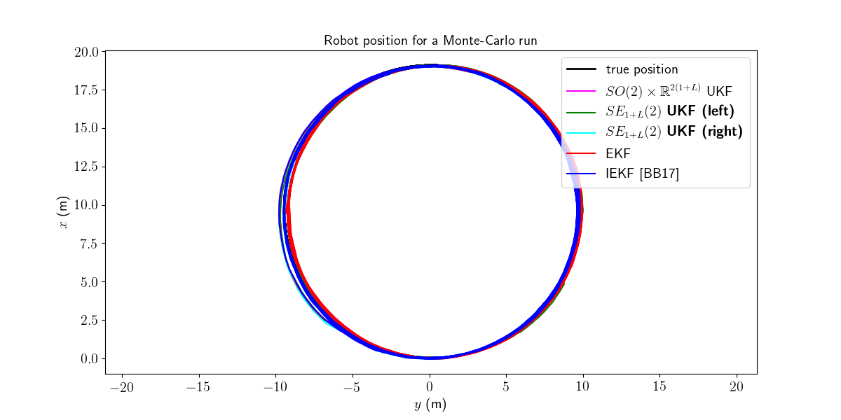
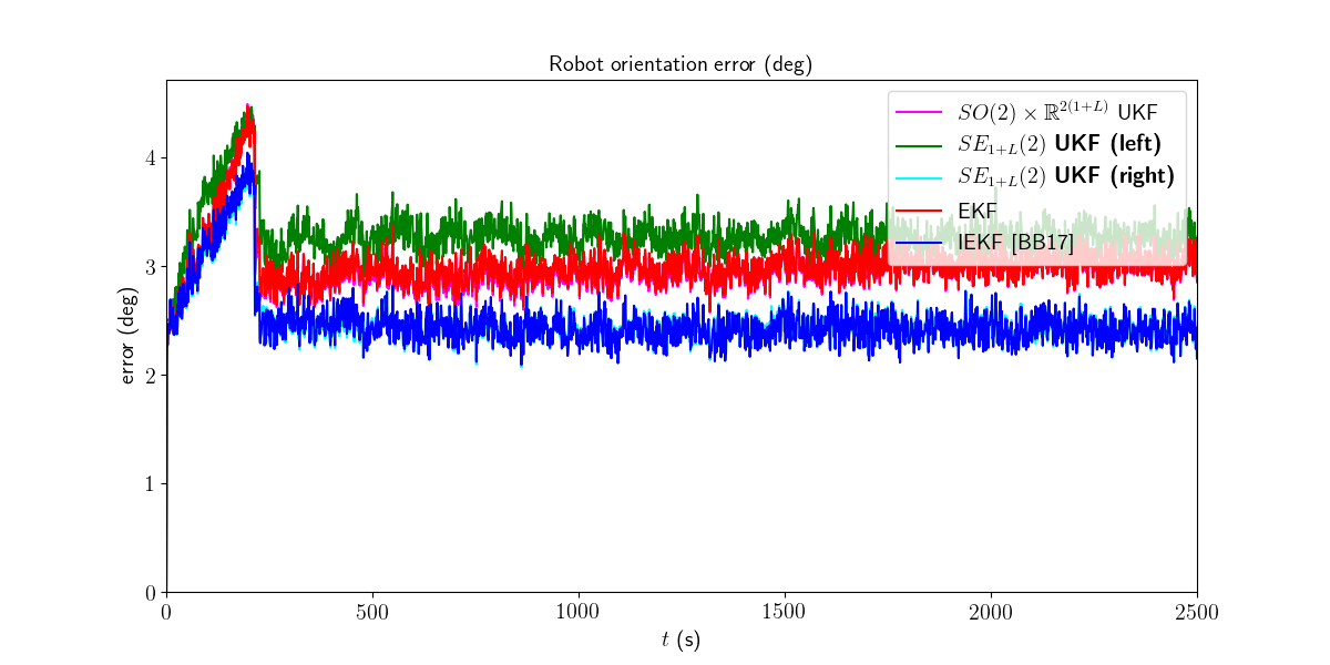
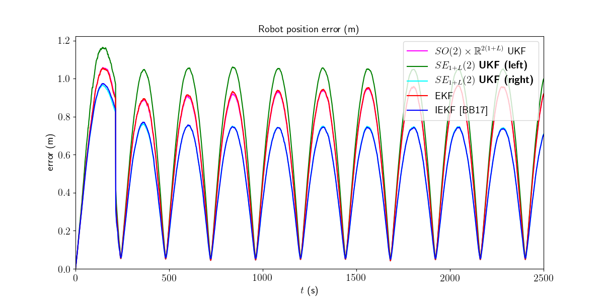
We first visualize the results for the last run, and then plot the orientation and position errors averaged over Monte-Carlo.
# get state
Rots, ps = model.get_states(states, model.N)
ukf_Rots, ukf_ps = model.get_states(ukf_states,  model.N)
left_ukf_Rots, left_ukf_ps = model.get_states(left_ukf_states,  model.N)
right_ukf_Rots, right_ukf_ps = model.get_states(right_ukf_states,  model.N)
iekf_Rots, iekf_ps = model.get_states(iekf_states,  model.N)
ekf_Rots, ekf_ps = model.get_states(ekf_states,  model.N)

ukf_err, left_ukf_err, right_ukf_err, iekf_err, ekf_err = model.benchmark_plot(
    ukf_err, left_ukf_err, right_ukf_err, iekf_err, ekf_err, ps, ukf_ps,
    left_ukf_ps, right_ukf_ps, ekf_ps, iekf_ps)
We then compute the Root Mean Squared Error (RMSE) for each method both for the orientation and the position.
model.benchmark_print(ukf_err, left_ukf_err, right_ukf_err, iekf_err, ekf_err)
Out:
Root Mean Square Error w.r.t. orientation (deg)
    -SO(2) x R^(2(1+L)) UKF: 3.01
    -left SE_{1+L}(2) UKF  : 3.30
    -right SE_{1+L}(2) UKF : 2.51
    -EKF                   : 3.02
    -IEKF                  : 2.51

Root Mean Square Error w.r.t. position (m)
    -SO(2) x R^(2(1+L)) UKF: 0.67
    -left SE_{1+L}(2) UKF  : 0.75
    -right SE_{1+L}(2) UKF : 0.55
    -EKF                   : 0.67
    -IEKF                  : 0.55
Right UKF and IEKF outperform the remaining filters.
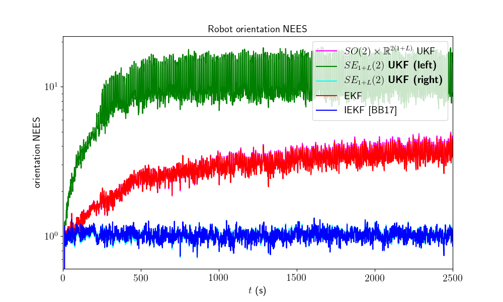
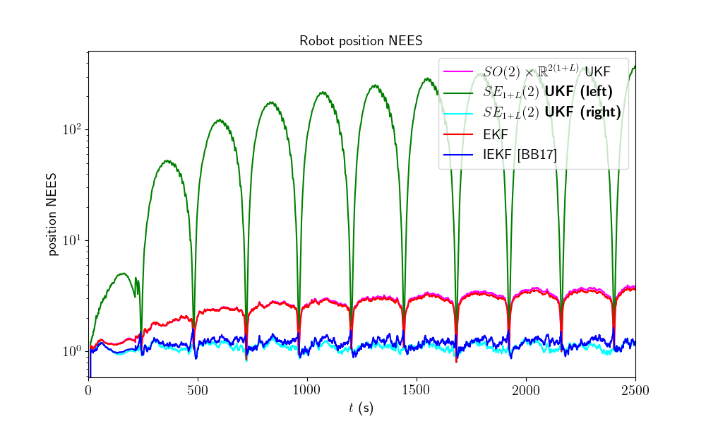
We now compare the filters in term of consistency (NEES).
model.nees_print(ukf_nees, left_ukf_nees, right_ukf_nees, iekf_nees, ekf_nees)
Out:
Normalized Estimation Error Squared (NEES) w.r.t. orientation
   -SO(2) x R^(2(1+L)) UKF:  2.93
   -left SE_{1+L}(2) UKF  :  10.38
   -right SE_{1+L}(2) UKF :  1.01
   -EKF                   :  2.88
   -IEKF                  :  1.01

Normalized Estimation Error Squared (NEES) w.r.t. position
   -SO(2) x R^(2(1+L)) UKF:  2.63
   -left SE_{1+L}(2) UKF  :  118.60
   -right SE_{1+L}(2) UKF :  1.09
   -EKF                   :  2.56
   -IEKF                  :  1.17
The right UKF and the IEKF obtain similar NEES and are the more consistent filters, whereas the remaining filter have their NEES increasing.
Which filter is the most accurate ? The right UKF and the IEKF are the best both in term of accuracy and consistency.
Conclusion
This script compares different algorithms for 2D robot SLAM. The right UKF and the IEKF are the more accurate filters. They are also consistent along all the trajectory.
You can now:
compare the filters in different scenarios. UKF and their (I)EKF counterparts may obtain different results when noise is inflated.
Total running time of the script: ( 248 minutes 35.587 seconds)
