Note
Click here to download the full example code
3D Attitude Estimation - Benchmark
Goals of this script:
implement two different UKFs on the 3D attitude estimation example.
design the Extended Kalman Filter (EKF).
compare the different algorithms with Monte-Carlo simulations.
We assume the reader is already familiar with the considered problem described in the related example.
For the given problem, two different UKFs emerge, defined respectively as:
1- The state is embedded in \(SO(3)\) with left multiplication, i.e.
the retraction \(\varphi(.,.)\) is the \(SO(3)\) exponential where uncertainty is multiplied on the left by the state.
the inverse retraction \(\varphi^{-1}(.,.)\) is the \(SO(3)\) logarithm.
2- The state is embedded in \(SO(3)\) with right multiplication, i.e.
the retraction \(\varphi(.,.)\) is the \(SO(3)\) exponential where uncertainty is multiplied on the right by the state.
the inverse retraction \(\varphi^{-1}(.,.)\) is the \(SO(3)\) logarithm.
We tests the different algorithms with the same noise parameter setting and on simulation with moderate initial heading error.
Import
from scipy.linalg import block_diag
from ukfm import SO3, UKF, EKF
from ukfm import ATTITUDE as MODEL
import ukfm
import numpy as np
import matplotlib
ukfm.set_matplotlib_config()
Simulation Setting
We compare the filters on a large number of Monte-Carlo runs.
# Monte-Carlo runs
N_mc = 100
This script uses the ATTITUDE() model. The initial values of the
heading error has 10° standard deviation.
# sequence time (s)
T = 100
# IMU frequency (Hz)
imu_freq = 100
# IMU noise standard deviation (noise is isotropic)
imu_std = np.array([5/180*np.pi,  # gyro (rad/s)
                    0.4,          # accelerometer (m/s**2)
                    0.3])         # magnetometer
# create the model
model = MODEL(T, imu_freq)
# propagation noise covariance matrix
Q = imu_std[0]**2*np.eye(3)
# measurement noise covariance matrix
R = block_diag(imu_std[1]**2*np.eye(3), imu_std[2]**2*np.eye(3))
# initial uncertainty matrix
P0 = (10/180*np.pi)**2*np.eye(3)  # The state is perfectly initialized
# sigma point parameters
alpha = np.array([1e-3, 1e-3, 1e-3])
Filter Design
Additionally to the UKFs, we compare them to an EKF. The EKF has the same uncertainty representation as the UKF with right uncertainty representation.
We set variables for recording metrics before launching Monte-Carlo simulations.
left_ukf_err = np.zeros((N_mc, model.N, 3))
right_ukf_err = np.zeros_like(left_ukf_err)
ekf_err = np.zeros_like(left_ukf_err)

left_ukf_nees = np.zeros((N_mc, model.N))
right_ukf_nees = np.zeros_like(left_ukf_nees)
ekf_nees = np.zeros_like(left_ukf_nees)
Monte-Carlo Runs
We run the Monte-Carlo through a for loop.
for n_mc in range(N_mc):
    print("Monte-Carlo iteration(s): " + str(n_mc+1) + "/" + str(N_mc))
    # simulate true states and noisy inputs
    states, omegas = model.simu_f(imu_std)
    # simulate accelerometer and magnetometer measurements
    ys = model.simu_h(states, imu_std)
    # initial state with error
    state0 = model.STATE(Rot=states[0].Rot.dot(
        SO3.exp(10/180*np.pi*np.random.randn(3))))
    # covariance need to be "turned"
    left_ukf_P = state0.Rot.dot(P0).dot(state0.Rot.T)
    right_ukf_P = P0
    ekf_P = P0

    # variables for recording estimates of the Monte-Carlo run
    left_ukf_states = [state0]
    right_ukf_states = [state0]
    ekf_states = [state0]

    left_ukf_Ps = np.zeros((model.N, 3, 3))
    right_ukf_Ps = np.zeros_like(left_ukf_Ps)
    ekf_Ps = np.zeros_like(left_ukf_Ps)

    left_ukf_Ps[0] = left_ukf_P
    right_ukf_Ps[0] = right_ukf_P
    ekf_Ps[0] = ekf_P

    left_ukf = UKF(state0=states[0], P0=P0, f=model.f, h=model.h, Q=Q, R=R,
                   phi=model.phi,
                   phi_inv=model.phi_inv,
                   alpha=alpha)
    right_ukf = UKF(state0=states[0], P0=P0, f=model.f, h=model.h, Q=Q, R=R,
                    phi=model.right_phi,
                    phi_inv=model.right_phi_inv,
                    alpha=alpha)
    ekf = EKF(model=model, state0=states[0], P0=P0, Q=Q, R=R,
              FG_ana=model.ekf_FG_ana,
              H_ana=model.ekf_H_ana,
              phi=model.right_phi)
    # filtering loop
    for n in range(1, model.N):
        # propagation
        left_ukf.propagation(omegas[n-1], model.dt)
        right_ukf.propagation(omegas[n-1], model.dt)
        ekf.propagation(omegas[n-1], model.dt)
        # update
        left_ukf.update(ys[n])
        right_ukf.update(ys[n])
        ekf.update(ys[n])
        # save estimates
        left_ukf_states.append(left_ukf.state)
        right_ukf_states.append(right_ukf.state)
        ekf_states.append(ekf.state)
        left_ukf_Ps[n] = left_ukf.P
        right_ukf_Ps[n] = right_ukf.P
        ekf_Ps[n] = ekf.P
    #  get state
    Rots, _ = model.get_states(states, model.N)
    left_ukf_Rots, _ = model.get_states(left_ukf_states, model.N)
    right_ukf_Rots, _ = model.get_states(right_ukf_states, model.N)
    ekf_Rots, _ = model.get_states(ekf_states, model.N)
    # record errors
    left_ukf_err[n_mc] = model.errors(Rots, left_ukf_Rots)
    right_ukf_err[n_mc] = model.errors(Rots, right_ukf_Rots)
    ekf_err[n_mc] = model.errors(Rots, ekf_Rots)
    # record NEES
    left_ukf_nees[n_mc] = model.nees(left_ukf_err[n_mc], left_ukf_Ps,
                                     left_ukf_Rots, 'LEFT')
    right_ukf_nees[n_mc] = model.nees(right_ukf_err[n_mc], right_ukf_Ps,
                                      right_ukf_Rots, 'RIGHT')
    ekf_nees[n_mc] = model.nees(ekf_err[n_mc], ekf_Ps, ekf_Rots, 'RIGHT')
Out:
Monte-Carlo iteration(s): 1/100
Monte-Carlo iteration(s): 2/100
Monte-Carlo iteration(s): 3/100
Monte-Carlo iteration(s): 4/100
Monte-Carlo iteration(s): 5/100
Monte-Carlo iteration(s): 6/100
Monte-Carlo iteration(s): 7/100
Monte-Carlo iteration(s): 8/100
Monte-Carlo iteration(s): 9/100
Monte-Carlo iteration(s): 10/100
Monte-Carlo iteration(s): 11/100
Monte-Carlo iteration(s): 12/100
Monte-Carlo iteration(s): 13/100
Monte-Carlo iteration(s): 14/100
Monte-Carlo iteration(s): 15/100
Monte-Carlo iteration(s): 16/100
Monte-Carlo iteration(s): 17/100
Monte-Carlo iteration(s): 18/100
Monte-Carlo iteration(s): 19/100
Monte-Carlo iteration(s): 20/100
Monte-Carlo iteration(s): 21/100
Monte-Carlo iteration(s): 22/100
Monte-Carlo iteration(s): 23/100
Monte-Carlo iteration(s): 24/100
Monte-Carlo iteration(s): 25/100
Monte-Carlo iteration(s): 26/100
Monte-Carlo iteration(s): 27/100
Monte-Carlo iteration(s): 28/100
Monte-Carlo iteration(s): 29/100
Monte-Carlo iteration(s): 30/100
Monte-Carlo iteration(s): 31/100
Monte-Carlo iteration(s): 32/100
Monte-Carlo iteration(s): 33/100
Monte-Carlo iteration(s): 34/100
Monte-Carlo iteration(s): 35/100
Monte-Carlo iteration(s): 36/100
Monte-Carlo iteration(s): 37/100
Monte-Carlo iteration(s): 38/100
Monte-Carlo iteration(s): 39/100
Monte-Carlo iteration(s): 40/100
Monte-Carlo iteration(s): 41/100
Monte-Carlo iteration(s): 42/100
Monte-Carlo iteration(s): 43/100
Monte-Carlo iteration(s): 44/100
Monte-Carlo iteration(s): 45/100
Monte-Carlo iteration(s): 46/100
Monte-Carlo iteration(s): 47/100
Monte-Carlo iteration(s): 48/100
Monte-Carlo iteration(s): 49/100
Monte-Carlo iteration(s): 50/100
Monte-Carlo iteration(s): 51/100
Monte-Carlo iteration(s): 52/100
Monte-Carlo iteration(s): 53/100
Monte-Carlo iteration(s): 54/100
Monte-Carlo iteration(s): 55/100
Monte-Carlo iteration(s): 56/100
Monte-Carlo iteration(s): 57/100
Monte-Carlo iteration(s): 58/100
Monte-Carlo iteration(s): 59/100
Monte-Carlo iteration(s): 60/100
Monte-Carlo iteration(s): 61/100
Monte-Carlo iteration(s): 62/100
Monte-Carlo iteration(s): 63/100
Monte-Carlo iteration(s): 64/100
Monte-Carlo iteration(s): 65/100
Monte-Carlo iteration(s): 66/100
Monte-Carlo iteration(s): 67/100
Monte-Carlo iteration(s): 68/100
Monte-Carlo iteration(s): 69/100
Monte-Carlo iteration(s): 70/100
Monte-Carlo iteration(s): 71/100
Monte-Carlo iteration(s): 72/100
Monte-Carlo iteration(s): 73/100
Monte-Carlo iteration(s): 74/100
Monte-Carlo iteration(s): 75/100
Monte-Carlo iteration(s): 76/100
Monte-Carlo iteration(s): 77/100
Monte-Carlo iteration(s): 78/100
Monte-Carlo iteration(s): 79/100
Monte-Carlo iteration(s): 80/100
Monte-Carlo iteration(s): 81/100
Monte-Carlo iteration(s): 82/100
Monte-Carlo iteration(s): 83/100
Monte-Carlo iteration(s): 84/100
Monte-Carlo iteration(s): 85/100
Monte-Carlo iteration(s): 86/100
Monte-Carlo iteration(s): 87/100
Monte-Carlo iteration(s): 88/100
Monte-Carlo iteration(s): 89/100
Monte-Carlo iteration(s): 90/100
Monte-Carlo iteration(s): 91/100
Monte-Carlo iteration(s): 92/100
Monte-Carlo iteration(s): 93/100
Monte-Carlo iteration(s): 94/100
Monte-Carlo iteration(s): 95/100
Monte-Carlo iteration(s): 96/100
Monte-Carlo iteration(s): 97/100
Monte-Carlo iteration(s): 98/100
Monte-Carlo iteration(s): 99/100
Monte-Carlo iteration(s): 100/100
Results
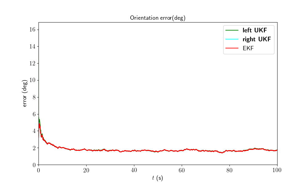
We visualize the results averaged over Monte-Carlo sequences, and compute the Root Mean Squared Error (RMSE) averaged over all Monte-Carlo.
model.benchmark_print(left_ukf_err, right_ukf_err, ekf_err)

Out:
Root Mean Square Error w.r.t. orientation (deg)
    -left UKF    : 1.06
    -right UKF   : 1.05
    -EKF         : 1.05
All the curves have the same shape. Filters obtain the same performances.
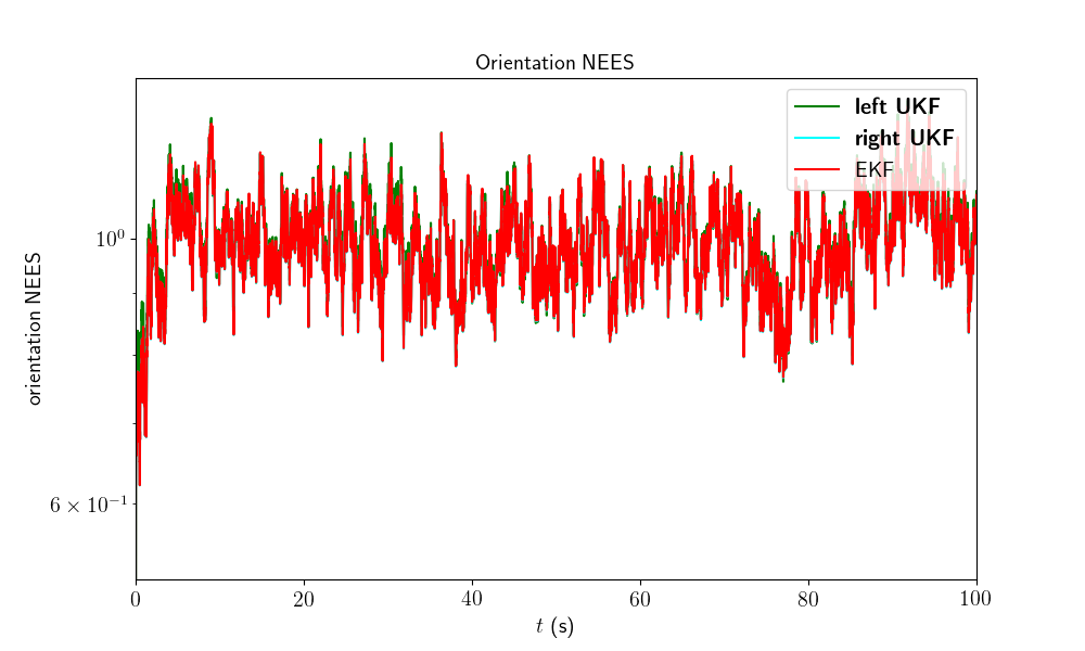
We finally compare the filters in term of consistency (Normalized Estimation Error Squared, NEES), as in the localization benchmark.
model.nees_print(left_ukf_nees, right_ukf_nees, ekf_nees)

Out:
Normalized Estimation Error Squared (NEES) w.r.t. orientation
   -left UKF    :  1.00
   -right UKF   :  0.99
   -EKF         :  0.99
All the filters obtain the same NEES and are consistent.
Which filter is the best ? For the considered problem, left UKF, right UKF, and EKF obtain the same performances. This is expected as when the state consists of an orientation only, left and right UKFs are implicitely the same. The EKF obtains similar results as it is also based on a retraction build on \(SO(3)\) (not with Euler angles).
Conclusion
This script compares two UKFs and one EKF for the problem of attitude estimation. All the filters obtain similar performances as the state involves only the orientation of the platform.
You can now:
compare the filters in different noise setting to see if the filters still get the same performances.
address the problem of 3D inertial navigation, where the state is defined as the oriention of the vehicle along with its velocity and its position.
Total running time of the script: ( 68 minutes 44.683 seconds)