2D Robot Localization on Real Data
Goals of this script:
- apply the UKF for the 2D robot localization example with real data.
We assume the reader is already familiar with the considered problem described in the tutorial.
We address the same problem as described in the tutorial on our own data.
Contents
Initialization
Start by cleaning the workspace.
clear all;
close all;
Model and Data
Instead of creating data, we load recorded data. We have recorded five sequences (sequence 2 and 3 are the more interesting).
% sequence number
n_sequence = 2;
% GPS frequency (Hz)
gps_freq = 2;
% GPS noise standard deviation (m)
gps_noise_std = 0.1;
% load data, where we simulation position measurement
[states, omegas, ys, one_hot_ys, t] = wifibot_load(n_sequence, gps_freq, ...
    gps_noise_std);
odo_noise_std = [0.15; % longitudinal speed
    0.05;              % transversal shift speed
    0.15];             % differential odometry
% total number of timestamps
N = length(states);
Filter Design and Initialization
We embed here the state in  with left multiplication.
% propagation noise covariance matrix
Q = diag(odo_noise_std.^2);
% measurement noise covariance matrix
R = gps_noise_std.^2 * eye(2);
% initial uncertainty matrix
P0 = zeros(3, 3);
% The state is not perfectly initialized
P0(1, 1) = (30/180*pi)^2;
% sigma point parameters
alpha = [1e-3, 1e-3, 1e-3];

% define the UKF propagation and measurement functions
f = @localization_f;
h = @localization_h;
phi = @localization_left_phi;
phi_inv = @localization_left_phi_inv;
% get UKF weight parameters
weights = ukf_set_weight(3, 2, alpha);
% compute Cholewski decomposition of Q only once
cholQ = chol(Q);
We initialize the filter with an initial heading error of 30°.
ukf_state = states(1);
% "add" orientation initial error
ukf_state.Rot = ukf_state.Rot * so2_exp(sqrt(P0(1, 1)));
ukf_P = P0;

% set variables for recording estimates along the full trajectory
ukf_states = ukf_state;
ukf_Ps = zeros(N, length(ukf_P), length(ukf_P));
ukf_Ps(1, :, :) = ukf_P;
Filtering
The UKF proceeds as a standard Kalman filter with a for loop.
% measurement iteration number (first measurement is for n == 1)
k = 2;
for n = 2:N
    % propagation
    dt = t(n) - t(n-1);
    Q = diag(odo_noise_std.^2);
    [ukf_state, ukf_P] = ukf_propagation(ukf_state, ukf_P, omegas(n-1), ...
        f, dt, phi, phi_inv, cholQ, weights);
    % update only if a measurement is received
    if one_hot_ys(n) == 1
       [ukf_state, ukf_P] = ukf_update(ukf_state, ukf_P, ys(:, k), ...
           h, phi, R, weights);
        k = k + 1;
    end
    % save estimates
    ukf_states(n) = ukf_state;
    ukf_Ps(n, :, :) = ukf_P;
end
Results
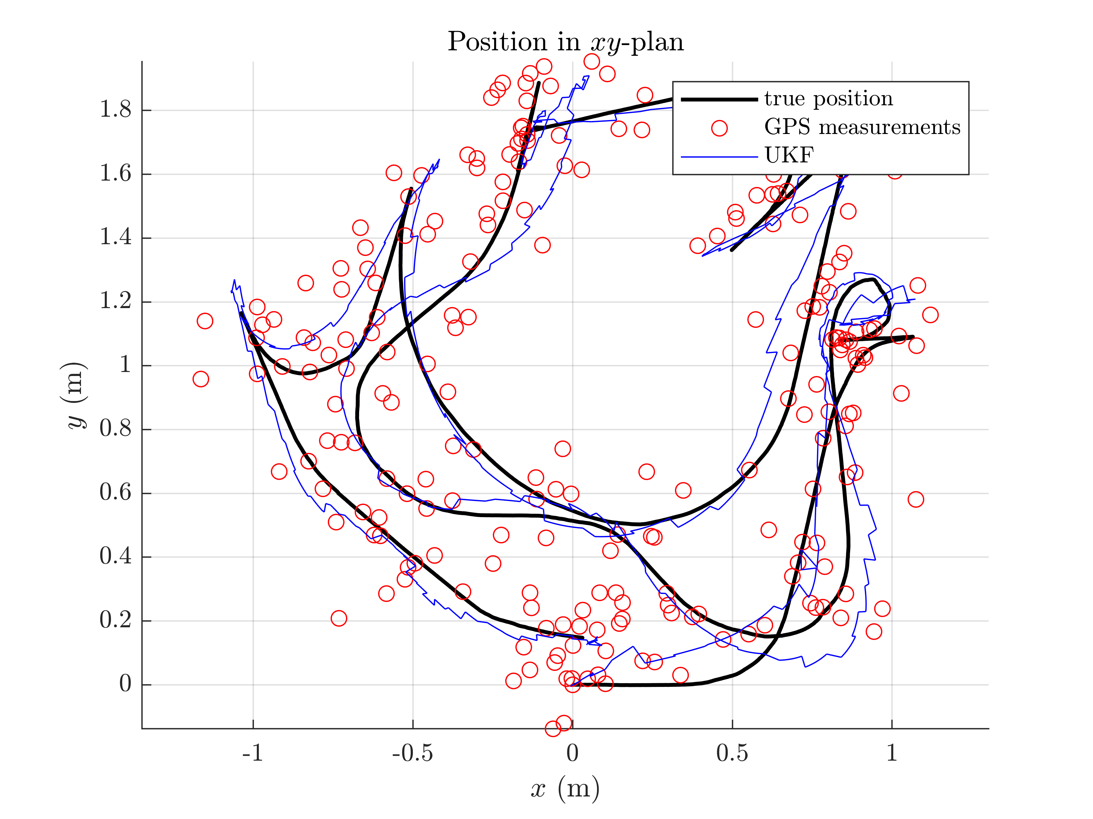
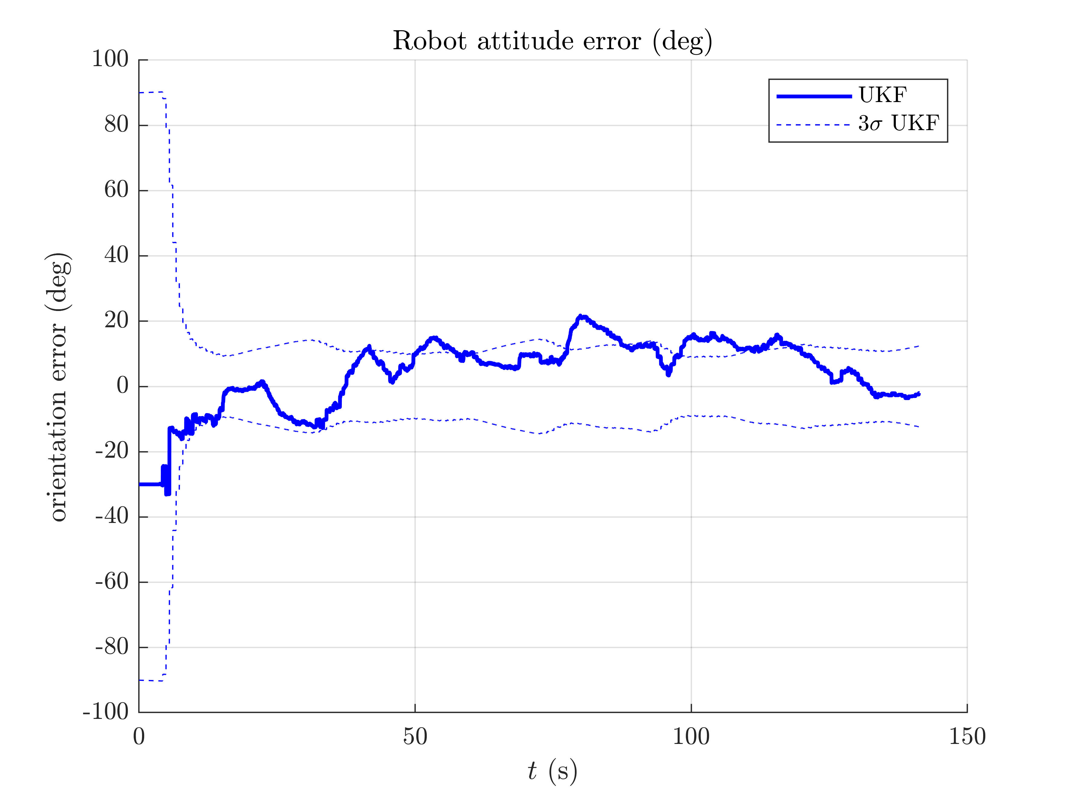
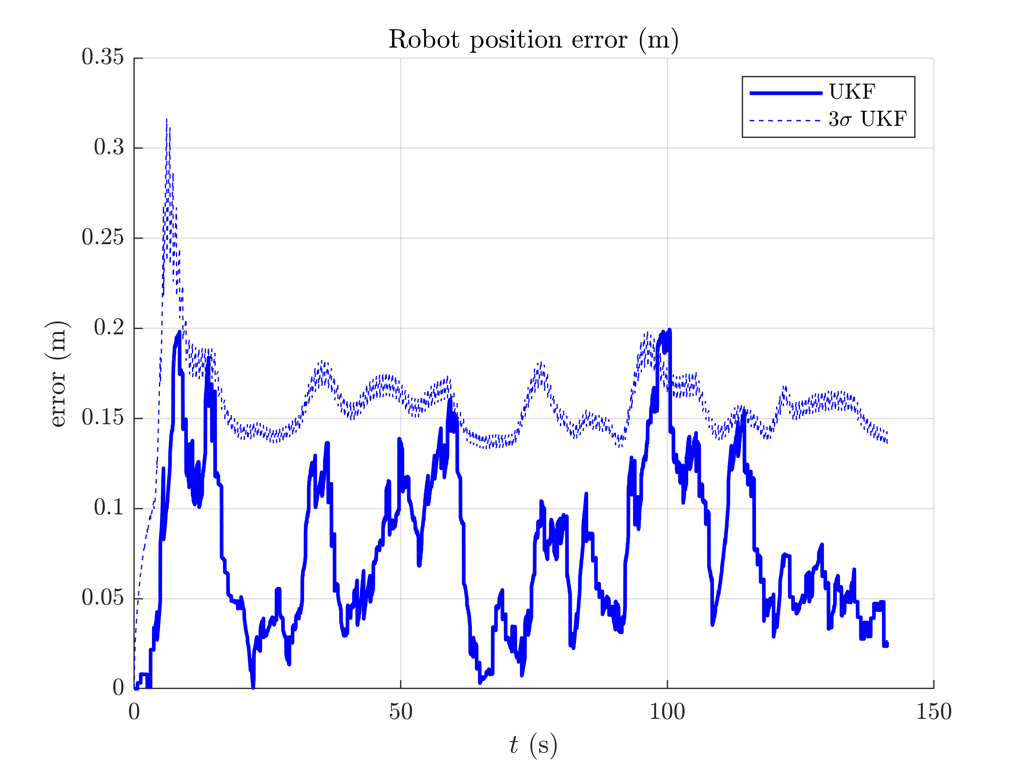
We plot the trajectory, the measurements and the estimated trajectory. We then plot the position and orientation error with 95% ( ) confident interval.
wifibot_results_plot(ukf_states, ukf_Ps, states, dt, ys);


All results are coherent. This is convincing as the initial heading error is relatively high.
Conclusion
This script applies the UKF for localizing a robot on real data. The filter works apparently well on this localization problem on real data, with moderate initial heading error.
You can now:
- test the UKF on different sequences.
- address the UKF for the same problem with range and bearing measurements of known landmarks.
- benchmark the UKF with different retractions and compare the new filters to both the extended Kalman filter and invariant extended Kalman filter of [BB17] (see the benchmarks section).