2D Robot Localization - Tutorial
This tutorial introduces the main aspects of UKF-M.
Goals of this script:
- understand the main principles of Unscented Kalman Filtering on Manifolds (UKF-M) [BBB19].
- get familiar with the implementation.
- design an UKF for a vanilla 2D robot localization problem.
We assume the reader to have sufficient prior knowledge with (unscented) Kalman filtering. However, we require really approximate prior knowledge and intuition about manifolds and tangent spaces.
This tutorial describes all one require to design an Unscented Kalman Filter (UKF) on a (parallelizable) manifold, and puts in evidence the versatility and simplicity of the method in term of implementation. Indeed, we need to define an UKF on parallelizable manifolds:
- a model of the state-space system that specifies the propagation and measurement functions of the system.
- an uncertainty representation of the estimated state, which is a mapping that generalizes the linear uncertainty definition
 .
. - standard UKF parameters that are noise covariance matrices and sigma point parameters.
We introduce the methodology by addressing the vanilla problem of robot localization, where the robot obtains velocity measurements, e.g., from wheel odometry, and position measurements, e.g., from GPS. The state consists of the robot orientation along with the 2D robot position. We reproduce the example described in [BB17], Section IV.
Contents
Initialization
Start by cleaning the workspace. Be also sure that all paths have been added, otherwise launch importukfm.m.
clear all;
close all;
The Model
The first ingredient we need is a model that defines:
- the state of the system at instant
 , noted
  , where
  is a parallelizable manifold (vectors spaces, Lie groups and others). Here the state corresponds to the robot orientation and the robot position.
 - a propagation function that describes how the state evolves along time.
- an observation function describing the measures we have.
We first define the model parameters.
% sequence time (s)
T = 40;
% odometry frequency (Hz)
odo_freq = 100;
% odometry noise standard deviation
odo_noise_std = [0.01;  % longitudinal speed (v/m)
    0.01;               % transversal shift speed (v/m)
    1/180*pi];          % differential odometry (rad/s)
% GPS frequency (Hz)
gps_freq = 1;
% GPS noise standard deviation (m)
gps_noise_std = 1;
% radius of the circle trajectory (m)
radius = 5;
% total number of timestamps
N = T*odo_freq;
% integration step (s)
dt = 1/odo_freq;
Simulating the Model
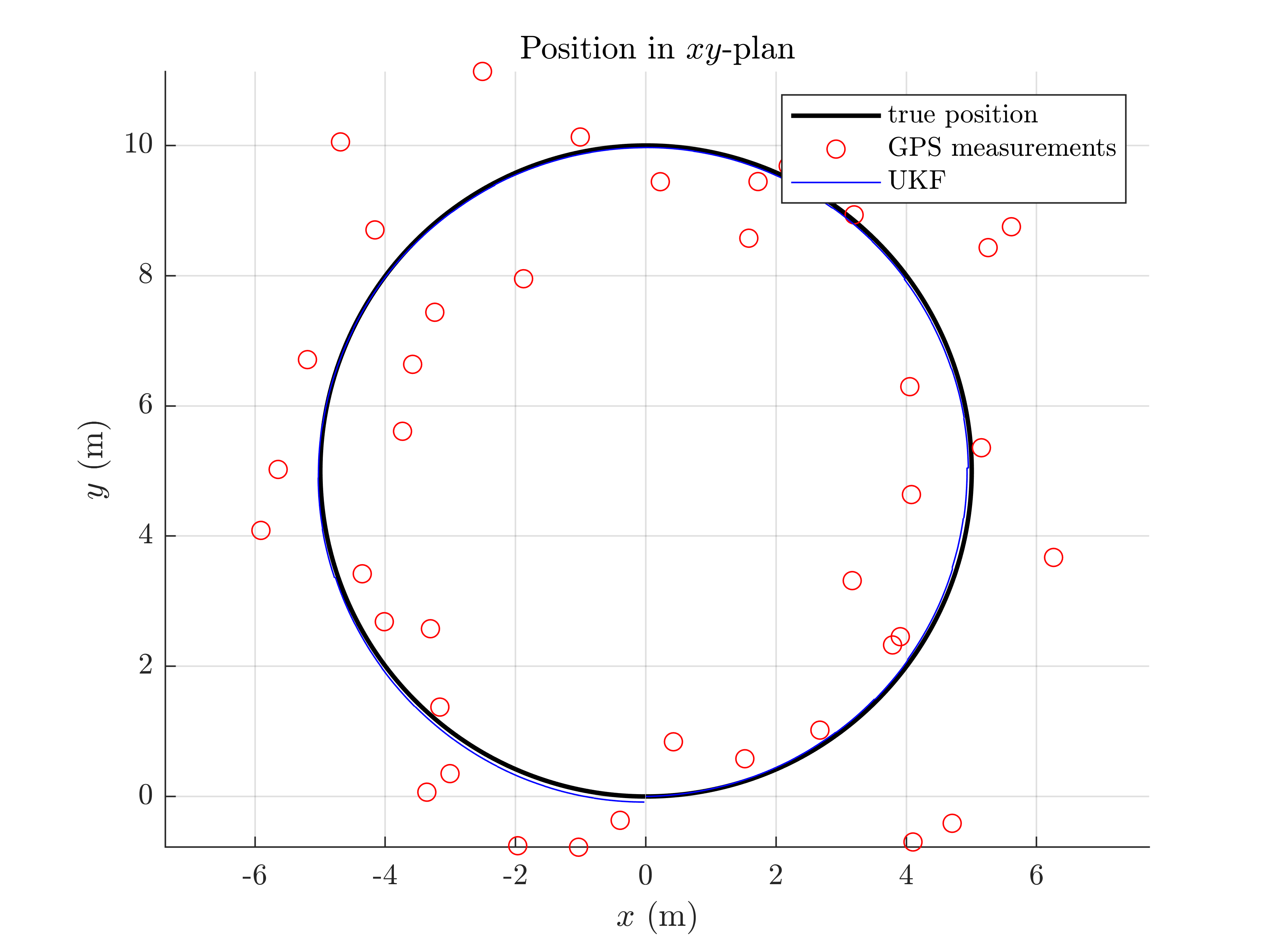
We compute simulated data, where the robot drives along a 10 m diameter circle for 40 seconds with high rate odometer measurements (100 Hz) and low rate position measurements (1 Hz). We obtain the true states along with noisy inputs.
[states, omegas] = localization_simu_f(T, odo_freq, odo_noise_std, radius);
The state and input are both array of structures. One can access to there values to a specific instant n as:
state = states(n)
omega = omegas(n)
We can then access to the elements of the state or the input as:
states(n).Rot         % 2d orientation encoded in a rotation matrix
states(n).p           % 2d position
omegas(n).v           % robot forward velocity
omegas(n).gyro        % robot angular velocity
The elements of the state and the input depend on the considered problem, where we encode the orientation in a rotation matrix. In all our examples, we define orientations in matrices living in  and
and  .
.
You can look at the localization folder to see the model function.
With the true state trajectory, we simulate noisy measurements.
[ys, one_hot_ys] = localization_simu_h(states, T, odo_freq, gps_freq, ...
    gps_noise_std);
 is a matrix that contains all the observations. To get the k-th measurement, take the k-th column as:
y = ys(:, k)
We have defined an array  that containts 1 at instant where a measurement happens and 0 otherwise.
Filter Design and Initialization
Designing an UKF on parallelizable manifolds consists in:
- defining a model of the propagation function and the measurement function.
- choosing the retraction
 and inverse retraction
  such that
  ,
,  , where
  is the true state,
  the estimated state, and
  the state uncertainty (we does not use notation
  and
and  to emphasize the differences with the linear case).
 - setting UKF parameters such as sigma point dispersion and noise covariance values.
Step 1) is already done, as we take the functions defined in the model.
Step 2) consists in choosing the mapping that encodes our representation of the state belief. A basic UKF is building on the uncertainty defined as  , which is not necessary optimal. Rather than, we define the uncertainty
  thought
  , where the retraction
  has to satisfy
  (without uncertainty, the estimated state equals the true state). We then need an inverse retraction to get a difference from two states that must respect
  .
.
We embed here the state in  , such that:
- the retraction
 is the
  exponential for orientation and the vector addition for position.
- the inverse retraction
 is the
  logarithm for orientation and the vector subtraction for position.
One can suggest alternative retractions, e.g. by viewing the state as a element of  . In the benchmarks folder, we compare different choices of retraction for different problems.
We know define UKF parameters, where we consider an innacurate initial heading estimation of 1°. We set the remaining filter parameters as in the model.
% propagation noise covariance matrix
Q = diag(odo_noise_std.^2);
% measurement noise covariance matrix
R = gps_noise_std.^2 * eye(2);
% initial uncertainty matrix
P0 = zeros(3, 3);
% The state is not perfectly initialized
P0(1, 1) = (1/180*pi)^2;
alpha = [1e-3, 1e-3, 1e-3];
% this parameter scales the sigma points. Current values are betwenn 10^-3 and 1

% define the UKF propagation and measurement functions
f = @localization_f;
h = @localization_h;
phi = @localization_phi;
phi_inv = @localization_phi_inv;
% get UKF weight parameters
weights = ukf_set_weight(3, 2, alpha);
% compute Cholewski decomposition of Q only once
cholQ = chol(Q);
We initialize the filter with the true state with a small error heading of 1°.
ukf_state = states(1);
% "add" orientation error to the initial state
ukf_state.Rot = ukf_state.Rot * so2_exp(sqrt(P0(1, 1)));
ukf_P = P0;

% set variables for recording estimates along the full trajectory
ukf_states = ukf_state;
ukf_Ps = zeros(N, length(ukf_P), length(ukf_P));
ukf_Ps(1, :, :) = ukf_P;
Filtering
The UKF proceeds as a standard Kalman filter with a for loop.
% measurement iteration number (first measurement is for n == 1)
k = 2;
for n = 2:N
    % propagation
    [ukf_state, ukf_P] = ukf_propagation(ukf_state, ukf_P, omegas(n-1), ...
        f, dt, phi, phi_inv, cholQ, weights);
    % update only if a measurement is received
    if one_hot_ys(n) == 1
        [ukf_state, ukf_P] = ukf_update(ukf_state, ukf_P, ys(:, k), ...
            h, phi, R, weights);
        k = k + 1;
    end
    % save estimates
    ukf_states(n) = ukf_state;
    ukf_Ps(n, :, :) = ukf_P;
end
Results
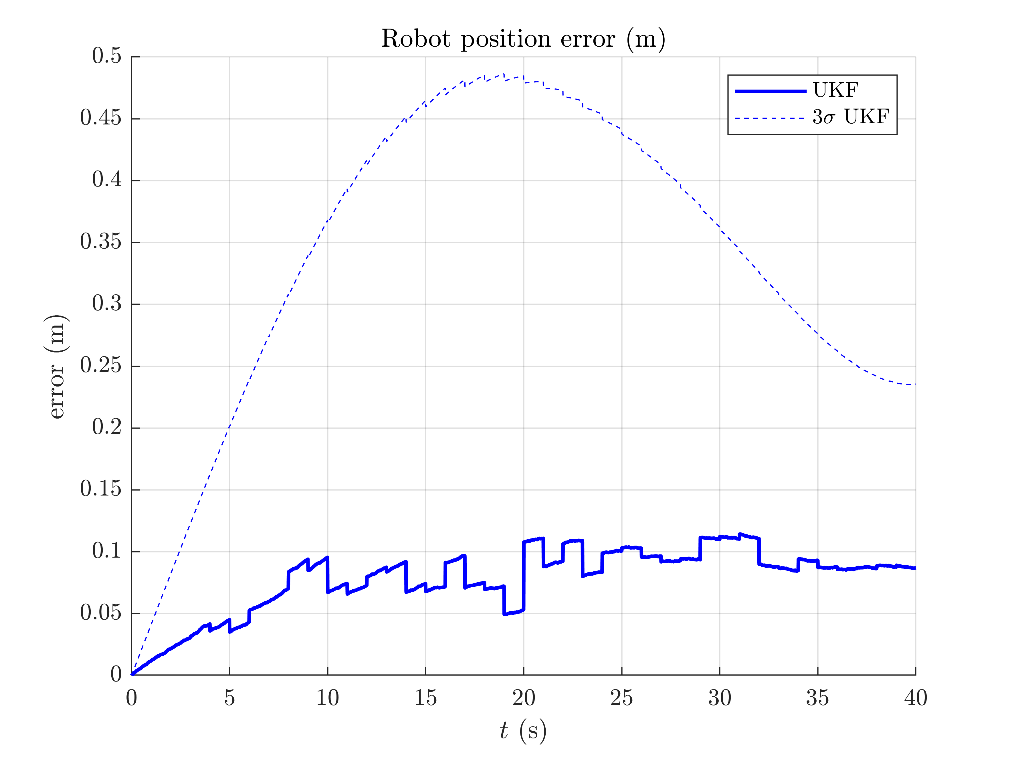
We plot the trajectory, GPS measurements and estimated trajectory. We then plot the orientation and position errors along with 95% ( ) confident interval. The results has to be confirmed with average metrics to reveal the filter performances in term of accuracy, consistency and robustness.
localization_results_plot(ukf_states, ukf_Ps, states, dt, ys);


All results seem coherent. This is expected as the initial heading error is small.
Conclusion
This script introduces UKF-M and shows how designing an UKF on parallelizable manifolds mainly consists in choosing an advantageous uncertainty representation. Two major interests of the method are that many problems could be addressed within the framework, and that both the theory and its implementation are sufficiently simple.
The filter works apparently well on a simple robot localization problem, with small initial heading error. Is it hold for more challenging initial error ?
You can now:
- enter more in depth with the theory, see [BBB19].
- address the UKF for the same problem with different noise parameters, and even test its robustness to strong initial heading error.
- modify the propagation model with a differential odometry model, where inputs are left and right wheel speed measurements.
- apply the UKF for the same problem on real data.
- benchmark the UKF with different retractions and compare the new filters to both the extended Kalman filter and invariant extended Kalman filter of [BB17].