Navigation on Flat Earth - Example

Goals of this script:

We assume the reader is already familiar with the approach described in the tutorial.

This script proposes an UKF on parallelizable manifolds to estimate the 3D attitude, the velocity, and the position of a rigid body in space from inertial sensors and relative observations of points having known locations by following the setting of [BB17] and [VCSO2010]. The vehicle is owed with a three axis Inertial Measurement Unit (IMU) consisting in accelerometers and gyroscopes. Observations of the relative position of known features (using for instance a depth camera) are addressed.

Contents

Initialization

Start by cleaning the workspace.

clear all;
close all;

Model and Simulation

% sequence time (s)
T = 30;
% IMU frequency (Hz)
imu_freq = 100;
% observation frequency (Hz)
obs_freq = 1;
% IMU noise standard deviation (noise is isotropic)
imu_noise_std = [0.01;  % gyro (rad/s)
                 0.01]; % accelerometer (m/s^2)
% number of observed landmarks
N_ldk = 3;
% observation noise standard deviation (m)
obs_noise_std = 0.1;
% total number of timestamps
N = T*imu_freq;
% integration step (s)
dt = 1/imu_freq;
% simulate true states and noisy inputs
[states, omegas] = inertial_navigation_simu_f(T, imu_freq, imu_noise_std);

The state and the input contain the following variables:

states(n).Rot      % 3d orientation (matrix)
states(n).v        % 3d velocity
states(n).p        % 3d position
omegas(n).gyro     % robot angular velocities
omegas(n).acc      % robot specific forces

We compute noisy measurements at low frequency based on the true states.

% simulate amers measurements
[ys, one_hot_ys] = inertial_navigation_simu_h(states, T, imu_freq, ...
    obs_freq, obs_noise_std);

A measurement ys(:, k) contains stacked observations of all visible landmarks.

Filter Design and Initilization

We now design the UKF on parallelizable manifolds. This script embeds the state in , such that:

Remaining parameter setting is standard. The initial errors are set around 10 degrees for attitude and 1 meter for position standard deviation. These initial conditions are challenging.

% propagation noise covariance matrix
Q = blkdiag(imu_noise_std(1)^2*eye(3), imu_noise_std(2)^2*eye(3));
% measurement noise covariance matrix
R = obs_noise_std.^2 * eye(3*N_ldk);
% initial uncertainty matrix such that the state is not perfectly initialized
P0 = blkdiag((10*pi/180)^2*eye(3), zeros(3, 3), eye(3));
% sigma point parameters
alpha = [1e-3, 1e-3, 1e-3];
% define the UKF functions
f = @inertial_navigation_f;
h = @inertial_navigation_h;
phi = @inertial_navigation_phi;
phi_inv = @inertial_navigation_phi_inv;
weights = ukf_set_weight(9, length(Q), alpha);
cholQ = chol(Q);
% initialize the filter
ukf_state = states(1);
ukf_state.Rot = so3_exp(pi/180*ones(3, 1)) * ukf_state.Rot;
ukf_state.p = ukf_state.p + [1;0.5;0.7];
ukf_P = P0;
% set variables for recording estimates along the full trajectory
ukf_states = ukf_state;
ukf_Ps = zeros(N, 9, 9);
ukf_Ps(1, :, :) = ukf_P;

Filtering

The UKF proceeds as a standard Kalman filter with a for loop.

% measurement iteration number
k = 2;
for n = 2:N
    % propagation
    [ukf_state, ukf_P] = ukf_propagation(ukf_state, ukf_P, omegas(n-1), ...
        f, dt, phi, phi_inv, cholQ, weights);
    % update only if a measurement is received
    if one_hot_ys(n) == 1
       [ukf_state, ukf_P] = ukf_update(ukf_state, ukf_P, ys(:, k), ...
           h, phi, R, weights);
        k = k + 1;
    end
    % save estimates
    ukf_states(n) = ukf_state;
    ukf_Ps(n, :, :) = ukf_P;
end

Results

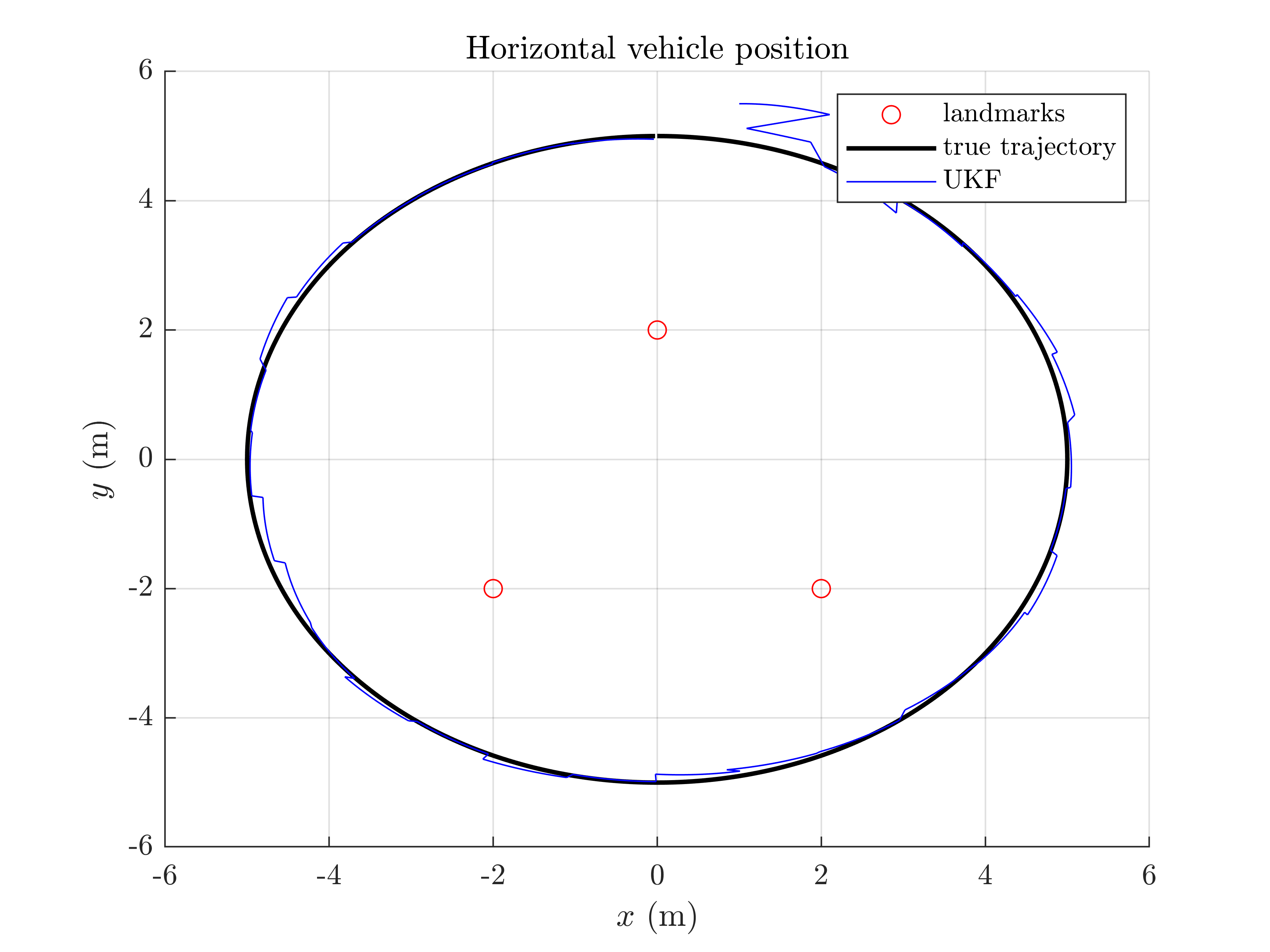
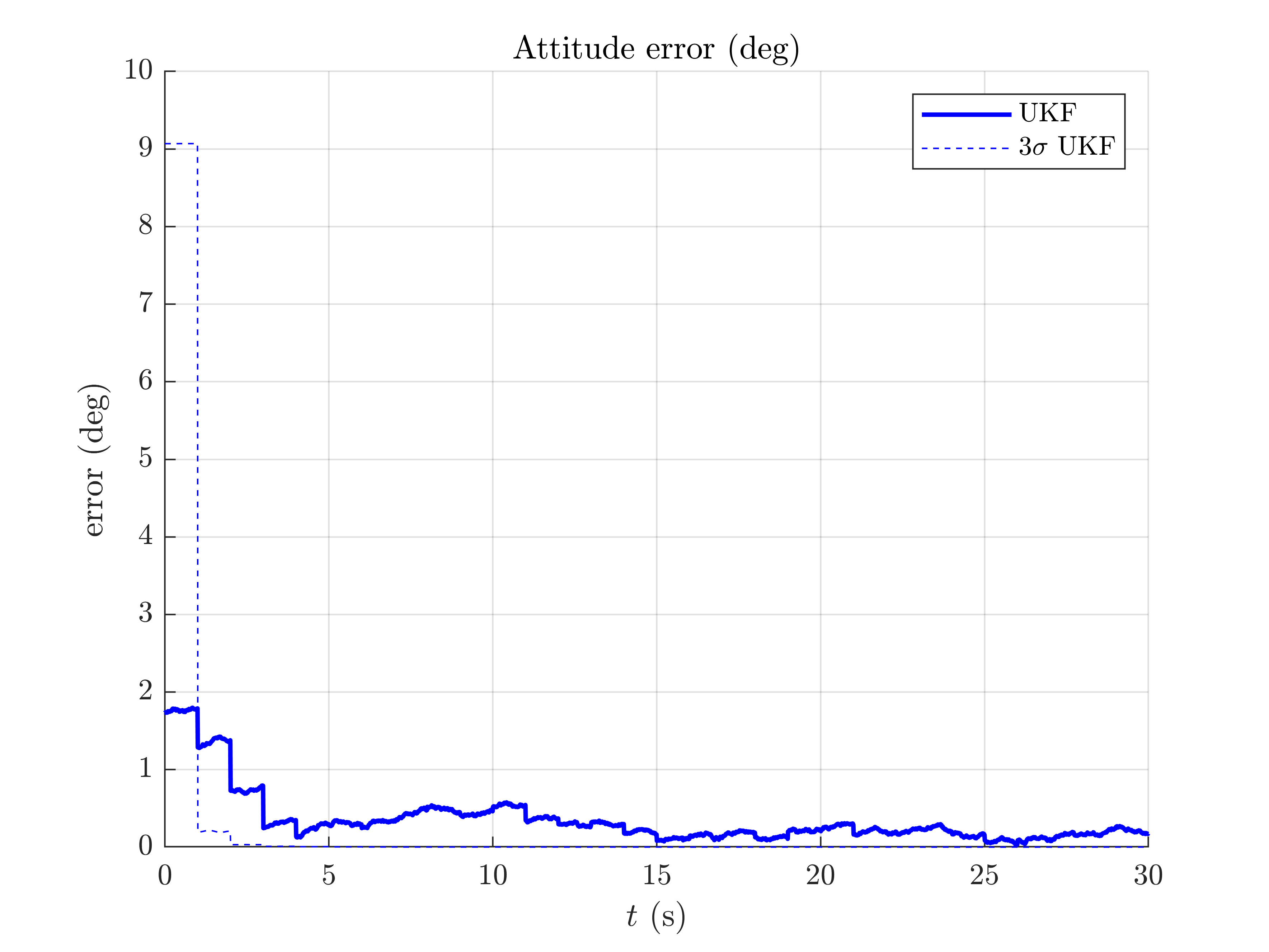
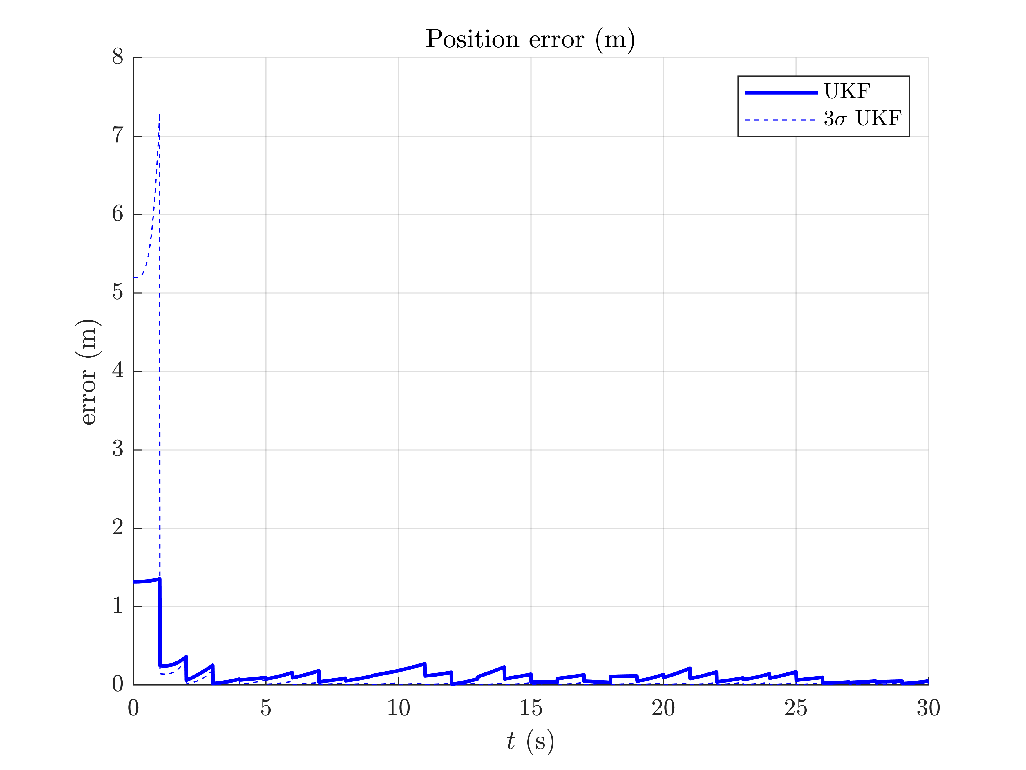
We plot the trajectory, the position of the landmarks and the estimated trajectory, along with attitude error, position error, and confidence interval.

inertial_navigation_results_plot(ukf_states, ukf_Ps, states, dt);

It seems that the proposed UKF meets strong difficulties and takes some time to converge due to the challenging initial conditions. A major problem of the UKF (in this problem and with this choice of retraction) is to be particularly overoptimism regarding attitude error, which is clearly outside the confidence intervals.

Conclusion

This script readily implements an UKF for estimation the 3D pose and velocity of a platform. Results are not particularly satisfying, since the filter difficultly converges to the true state even at the end of the trajectory. But is it not possible to improve the filter accuracy and consistency performances by inflating sensor noise parameters of the filter, or better, by defining a retraction more adapted to the considered problem ?

You can now:

Published with MATLAB® R2019a