2D Robot Localization - Benchmark
Goals of this script:
- implement different UKFs on the 2D robot localization example.
- design the Extended Kalman Filter (EKF) and the Invariant Extended Kalman Filter (IEKF) [BB17].
- compare the different algorithms with Monte-Carlo simulations.
We assume the reader is already familiar with the considered problem described in the tutorial.
We previously designed an UKF with a standard uncertainty representation. An advantage of the versatility of the UKF is to speed up implementation, tests, and comparision UKF with different uncertainty representations. Indeed, for the given problem, three different UKFs emerge, defined respectively as:
- The state is embedded in
 , where: the retraction
  is the
  exponential for orientation and the vector addition for position; the inverse retraction
  is the
  logarithm for orientation and the vector subtraction for position.
 - The state is embedded in
 with left multiplication, i.e. the retraction
  is the
  exponential, where the state multiplies on the left the uncertainty
  . The inverse retraction
  is the
  logarithm. This left UKF on
  corresponds to the Invariant Extended Kalman Filter (IEKF) recommended in [BB17].
 - The state is embedded in
 with right multiplication, i.e. the retraction
  is the
  exponential, where the state multiplies on the right the uncertainty
  . The inverse retraction
  is the
  logarithm.
We tests the filters on simulation with strong initial heading error.
Contents
Initialization
Start by cleaning the workspace.
clear all;
close all;
We compare the filters on a large number of Monte-Carlo runs.
% Monte-Carlo runs
N_mc = 100;
Simulation Settion
We set the simulation as in [BB17], section IV. The robot drives along a 10 m diameter circle for 40 seconds with high rate odometer measurements (100 Hz) and low rate GPS measurements (1 Hz). The vehicle gets moderate angular velocity uncertainty and highly precise linear velocity. The initial values of the heading error is very strong, 45° standard deviation , while the initial position is known.
% sequence time (s)
T = 40;
% odometry frequency (Hz)
odo_freq = 100;
% odometry noise standard deviation
odo_noise_std = [0.01; % speed (v/m)
                 0.01; % speed (v/m)
                 1/180*pi]; % angular speed (rad/s)
% GPS frequency (Hz)
gps_freq = 1;
% GPS noise standard deviation (m)
gps_noise_std = 1;
% total number of timestamps
N = T*odo_freq;
% integration step (s)
dt = 1/odo_freq;
% radius of the circle trajectory (m)
radius = 5;
Filter Design
Additionally to the three UKFs, we compare them to an Extended Kalman FIlter (EKF) and an Invariant EKF (IEKF). The EKF has the same uncertainty representation as the UKF with the retraction on  , whereas the IEKF has the same uncertainty representation as the UKF with the left retraction on
  .
.
% propagation noise covariance matrix
Q = diag(odo_noise_std.^2);
% measurement noise covariance matrix
R = gps_noise_std^2 * eye(2);
% initial uncertainty matrix
P0 = zeros(3, 3);
init_heading_error_std = 45/180*pi;
% we take into account initial heading error
P0(1, 1) = (init_heading_error_std)^2;
% sigma point parameter
alpha = [1e-3 1e-3 1e-3];

% define the UKF functions
f = @localization_f;
h = @localization_h;

phi = @localization_phi;
left_phi = @localization_left_phi;
right_phi = @localization_right_phi;

phi_inv = @localization_phi_inv;
left_phi_inv = @localization_left_phi_inv;
right_phi_inv = @localization_right_phi_inv;

weights = ukf_set_weight(length(P0), length(Q), alpha);
cholQ = chol(Q);
We set error variables before launching Monte-Carlo simulations. As we have five similar methods, the code is redundant.
ukf_errs = zeros(3, N, N_mc);
ukf_left_errs = zeros(size(ukf_errs));
ukf_right_errs = zeros(size(ukf_errs));
iekf_errs = zeros(size(ukf_errs));
ekf_errs = zeros(size(ukf_errs));
We record Normalized Estimation Error Squared (NEES) for consistency evaluation (see Results section).
ukf_nees = zeros(2, N, N_mc);
left_ukf_nees = zeros(size(ukf_nees));
right_ukf_nees = zeros(size(ukf_nees));
iekf_nees = zeros(size(ukf_nees));
ekf_nees = zeros(size(ukf_nees));
Monte-Carlo runs
We run the Monte-Carlo through a for loop.
for n_mc = 1:N_mc
    disp("Monte-Carlo iteration(s): " + num2str(n_mc) + "/" + num2str(N_mc));
    % simulation true states
    [states, omegas] = localization_simu_f(T, odo_freq, odo_noise_std, ...
        radius);
    % simulate measurements
    [ys, one_hot_ys] = localization_simu_h(states, T, odo_freq, gps_freq, ...
        gps_noise_std);
    % initialize filter with innacurate state
    ukf_state = states(1);
    % we sample an initial heading error from the true distribution.
    init_heading_error = init_heading_error_std*randn(1);
    ukf_state.Rot = states(1).Rot * so2_exp(init_heading_error);
    ukf_left_state = ukf_state(1);
    ukf_right_state = ukf_state(1);
    ekf_state = ukf_state(1);
    iekf_state = ukf_state(1);

    ukf_P = P0;
    ukf_left_P = P0;
    ukf_right_P = P0;
    ekf_P = P0;
    iekf_P = P0;

    % variables for recording estimates of the Monte-Carlo run
    ukf_states = ukf_state;
    ukf_left_states = ukf_left_state;
    ukf_right_states = ukf_right_state;
    iekf_states = iekf_state;
    ekf_states = ekf_state;

    ukf_Ps = zeros(N, 3, 3);
    ukf_left_Ps = zeros(size(ukf_Ps));
    ukf_right_Ps = zeros(size(ukf_Ps));
    ekf_Ps = zeros(size(ukf_Ps));
    iekf_Ps = zeros(size(ukf_Ps));

    ukf_Ps(1, :, :) = ukf_P;
    ukf_left_Ps(1, :, :) = ukf_left_P;
    ukf_right_Ps(1, :, :) = ukf_right_P;
    ekf_Ps(1, :, :) = ekf_P;
    iekf_Ps(1, :, :) = iekf_P;

    % measurement iteration number
    k = 2;
    % filtering loop
    for n = 2:N
        % propagation
        [ukf_state, ukf_P] = ukf_propagation(ukf_state, ukf_P, omegas(n-1), ...
            f, dt, phi, phi_inv, cholQ, weights);
        [ukf_left_state, ukf_left_P] = ukf_propagation(ukf_left_state, ...
            ukf_left_P, omegas(n-1), f, dt, left_phi, ...
            left_phi_inv, cholQ, weights);
        [ukf_right_state, ukf_right_P] = ukf_propagation(ukf_right_state, ...
            ukf_right_P, omegas(n-1), f, dt, right_phi, right_phi_inv, ...
            cholQ, weights);
        [ekf_state, ekf_P] = localization_ekf_propagation(ekf_state, ...
            ekf_P, omegas(n-1), dt, Q);
        [iekf_state, iekf_P] = localization_iekf_propagation(...
            iekf_state, iekf_P, omegas(n-1), dt, Q);

        % update only if a measurement is received
        if one_hot_ys(n) == 1
           [ukf_state, ukf_P] = ukf_update(ukf_state, ukf_P, ys(:, k), ...
               h, phi, R, weights);
           [ukf_left_state, ukf_left_P] = ukf_update(ukf_left_state, ...
               ukf_left_P, ys(:, k), h, left_phi, R, weights);
           [ukf_right_state, ukf_right_P] = ukf_update(ukf_right_state, ...
               ukf_right_P, ys(:, k), h, right_phi, R, weights);
           [ekf_state, ekf_P] = localization_ekf_update(ekf_state, ...
               ekf_P, ys(:, k), R);
           [iekf_state, iekf_P] = localization_iekf_update(iekf_state, ...
               iekf_P, ys(:, k), R);
            k = k + 1;
        end
        % save estimates
        ukf_states(n) = ukf_state;
        ukf_left_states(n) = ukf_left_state;
        ukf_right_states(n) = ukf_right_state;
        ekf_states(n) = ekf_state;
        iekf_states(n) = iekf_state;

        ukf_Ps(n, :, :) = ukf_P;
        ukf_left_Ps(n, :, :) = ukf_left_P;
        ukf_right_Ps(n, :, :) = ukf_right_P;
        ekf_Ps(n, :, :) = ekf_P;
        iekf_Ps(n, :, :) = iekf_P;
    end
    % get state trajectory
    [Rots, ps] = localization_get_states(states);
    [ukf_Rots, ukf_ps] = localization_get_states(ukf_states);
    [ukf_left_Rots, ukf_left_ps] = localization_get_states(ukf_left_states);
    [ukf_right_Rots, ukf_right_ps] = localization_get_states(ukf_right_states);
    [iekf_Rots, iekf_ps] = localization_get_states(iekf_states);
    [ekf_Rots, ekf_ps] = localization_get_states(ekf_states);

    % record errors
    ukf_errs(:, :, n_mc) = localization_errors(Rots, ukf_Rots, ps, ukf_ps);
    ukf_left_errs(:, :, n_mc) = localization_errors(Rots, ukf_left_Rots, ps, ...
        ukf_left_ps);
    ukf_right_errs(:, :, n_mc) = localization_errors(Rots, ukf_right_Rots, ...
        ps, ukf_right_ps);
    iekf_errs(:, :, n_mc) = localization_errors(Rots, iekf_Rots, ps, iekf_ps);
    ekf_errs(:, :, n_mc) = localization_errors(Rots, ekf_Rots, ps, ekf_ps);

    % record NEES
    ukf_nees(:, :, n_mc) = localization_nees(ukf_errs(:, :, n_mc), ukf_Ps, ...
        ukf_Rots, ukf_ps, "STD");
    ukf_left_nees(:, :, n_mc) = localization_nees(ukf_left_errs(:, :, n_mc), ...
        ukf_left_Ps, ukf_left_Rots, ukf_left_ps, "LEFT");
    ukf_right_nees(:, :, n_mc) = localization_nees(...
        ukf_right_errs(:, :, n_mc), ukf_right_Ps, ukf_right_Rots, ...
        ukf_right_ps, "RIGHT");
    iekf_nees(:, :, n_mc) = localization_nees(iekf_errs(:, :, n_mc), iekf_Ps, ...
        iekf_Rots, iekf_ps, "LEFT");
    ekf_nees(:, :, n_mc) = localization_nees(ekf_errs(:, :, n_mc), ekf_Ps, ...
        ekf_Rots, ekf_ps, "STD");
end
Monte-Carlo iteration(s): 1/100
Monte-Carlo iteration(s): 2/100
Monte-Carlo iteration(s): 3/100
Monte-Carlo iteration(s): 4/100
Monte-Carlo iteration(s): 5/100
Monte-Carlo iteration(s): 6/100
Monte-Carlo iteration(s): 7/100
Monte-Carlo iteration(s): 8/100
Monte-Carlo iteration(s): 9/100
Monte-Carlo iteration(s): 10/100
Monte-Carlo iteration(s): 11/100
Monte-Carlo iteration(s): 12/100
Monte-Carlo iteration(s): 13/100
Monte-Carlo iteration(s): 14/100
Monte-Carlo iteration(s): 15/100
Monte-Carlo iteration(s): 16/100
Monte-Carlo iteration(s): 17/100
Monte-Carlo iteration(s): 18/100
Monte-Carlo iteration(s): 19/100
Monte-Carlo iteration(s): 20/100
Monte-Carlo iteration(s): 21/100
Monte-Carlo iteration(s): 22/100
Monte-Carlo iteration(s): 23/100
Monte-Carlo iteration(s): 24/100
Monte-Carlo iteration(s): 25/100
Monte-Carlo iteration(s): 26/100
Monte-Carlo iteration(s): 27/100
Monte-Carlo iteration(s): 28/100
Monte-Carlo iteration(s): 29/100
Monte-Carlo iteration(s): 30/100
Monte-Carlo iteration(s): 31/100
Monte-Carlo iteration(s): 32/100
Monte-Carlo iteration(s): 33/100
Monte-Carlo iteration(s): 34/100
Monte-Carlo iteration(s): 35/100
Monte-Carlo iteration(s): 36/100
Monte-Carlo iteration(s): 37/100
Monte-Carlo iteration(s): 38/100
Monte-Carlo iteration(s): 39/100
Monte-Carlo iteration(s): 40/100
Monte-Carlo iteration(s): 41/100
Monte-Carlo iteration(s): 42/100
Monte-Carlo iteration(s): 43/100
Monte-Carlo iteration(s): 44/100
Monte-Carlo iteration(s): 45/100
Monte-Carlo iteration(s): 46/100
Monte-Carlo iteration(s): 47/100
Monte-Carlo iteration(s): 48/100
Monte-Carlo iteration(s): 49/100
Monte-Carlo iteration(s): 50/100
Monte-Carlo iteration(s): 51/100
Monte-Carlo iteration(s): 52/100
Monte-Carlo iteration(s): 53/100
Monte-Carlo iteration(s): 54/100
Monte-Carlo iteration(s): 55/100
Monte-Carlo iteration(s): 56/100
Monte-Carlo iteration(s): 57/100
Monte-Carlo iteration(s): 58/100
Monte-Carlo iteration(s): 59/100
Monte-Carlo iteration(s): 60/100
Monte-Carlo iteration(s): 61/100
Monte-Carlo iteration(s): 62/100
Monte-Carlo iteration(s): 63/100
Monte-Carlo iteration(s): 64/100
Monte-Carlo iteration(s): 65/100
Monte-Carlo iteration(s): 66/100
Monte-Carlo iteration(s): 67/100
Monte-Carlo iteration(s): 68/100
Monte-Carlo iteration(s): 69/100
Monte-Carlo iteration(s): 70/100
Monte-Carlo iteration(s): 71/100
Monte-Carlo iteration(s): 72/100
Monte-Carlo iteration(s): 73/100
Monte-Carlo iteration(s): 74/100
Monte-Carlo iteration(s): 75/100
Monte-Carlo iteration(s): 76/100
Monte-Carlo iteration(s): 77/100
Monte-Carlo iteration(s): 78/100
Monte-Carlo iteration(s): 79/100
Monte-Carlo iteration(s): 80/100
Monte-Carlo iteration(s): 81/100
Monte-Carlo iteration(s): 82/100
Monte-Carlo iteration(s): 83/100
Monte-Carlo iteration(s): 84/100
Monte-Carlo iteration(s): 85/100
Monte-Carlo iteration(s): 86/100
Monte-Carlo iteration(s): 87/100
Monte-Carlo iteration(s): 88/100
Monte-Carlo iteration(s): 89/100
Monte-Carlo iteration(s): 90/100
Monte-Carlo iteration(s): 91/100
Monte-Carlo iteration(s): 92/100
Monte-Carlo iteration(s): 93/100
Monte-Carlo iteration(s): 94/100
Monte-Carlo iteration(s): 95/100
Monte-Carlo iteration(s): 96/100
Monte-Carlo iteration(s): 97/100
Monte-Carlo iteration(s): 98/100
Monte-Carlo iteration(s): 99/100
Monte-Carlo iteration(s): 100/100
Results
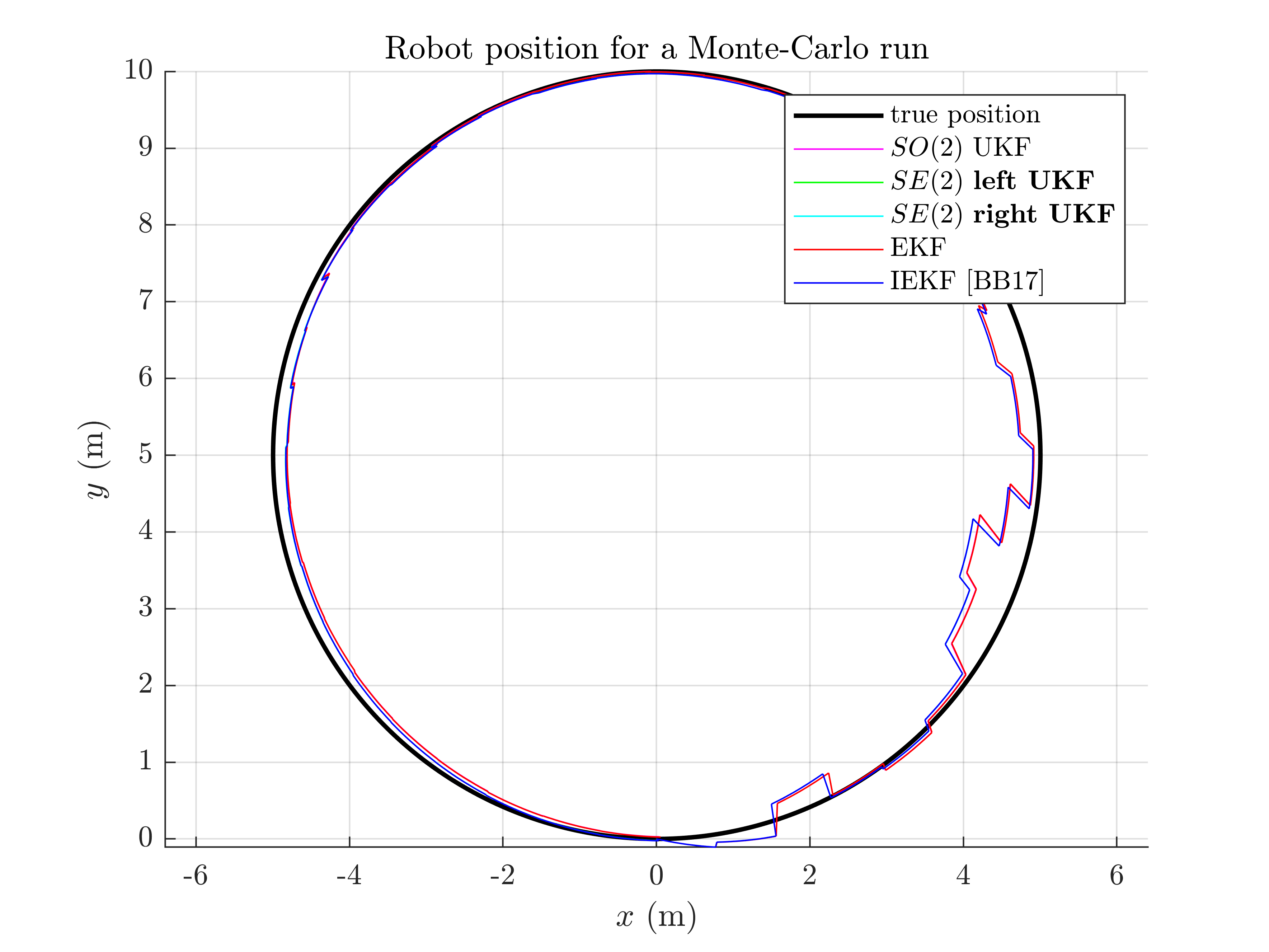
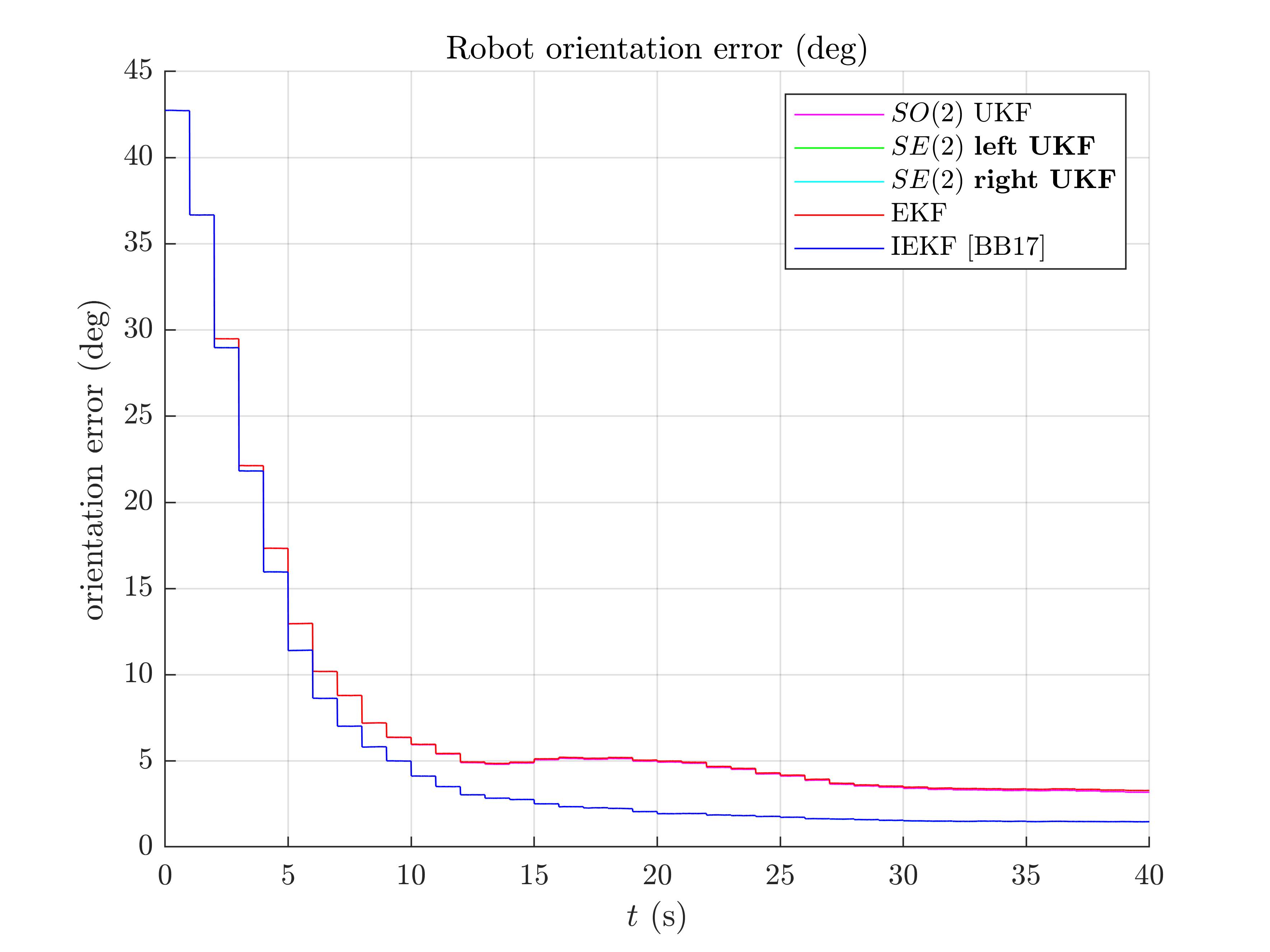
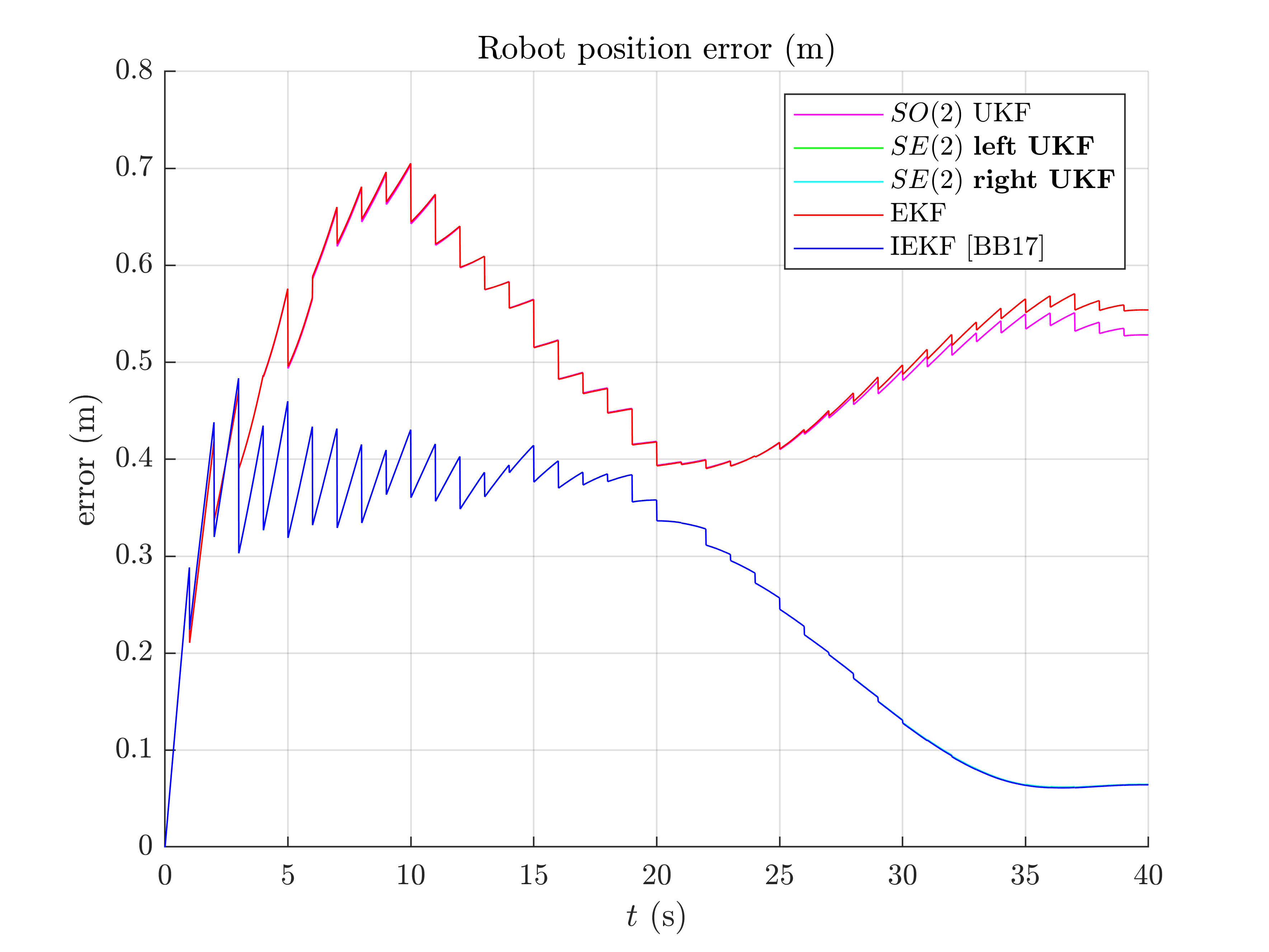
Once simulations are done, we compare the algorithms. Let us first visualize the results in term of estimated robot trajectory (for the last run) and the errors w.r.t. orientation and position (averaged over Monte-Carlo). As simulations have random process, the trajectory plot just gives us an indication but not a proof of performances.
We then compute the Root Mean Squared Error (RMSE) for each method both for the orientation and the position.
benchmark_localization_helper;
Root Mean Square Error w.r.t. orientation (deg)
    -SO(2) x R^2 UKF: 12.07
    -left SE(2) UKF : 11.39
    -right SE(2) UKF: 11.39
    -EKF            : 12.08
    -IEKF           : 11.39

Root Mean Square Error w.r.t. position (m)
    -SO(2) x R^2 UKF: 0.51
    -left SE(2) UKF : 0.30
    -right SE(2) UKF: 0.30
    -EKF            : 0.51
    -IEKF           : 0.29


A statement seem obvious, we have two groups of filters: group 1) consists of EKF and  UKF; and group 2) have IEKF, left
  UKF and right
  UKF (the curves of these filters are superposed). The second group is visibly highly better regarding position estimation.
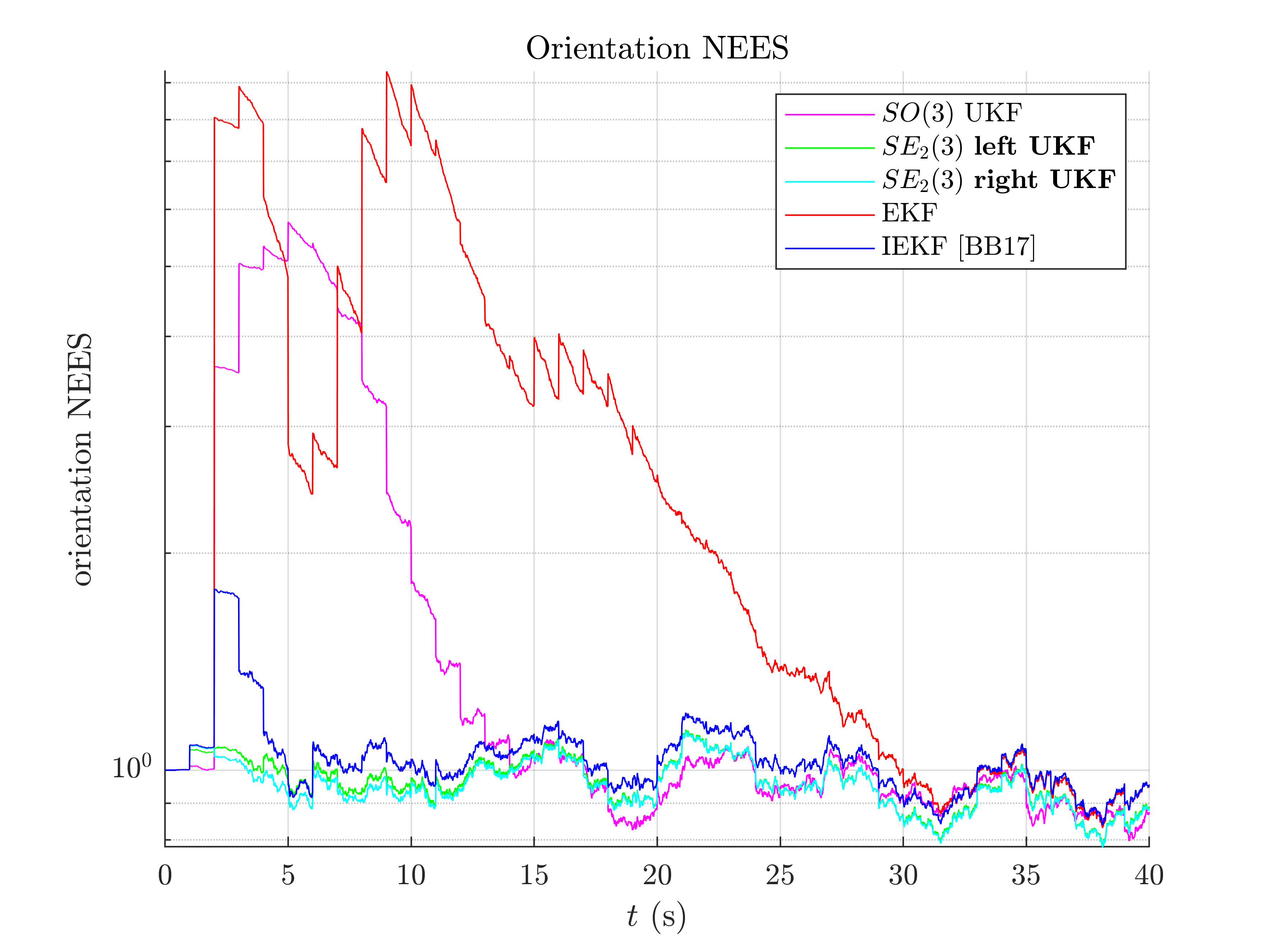
A consistency metric is the Normalized Estimation Error Squared (NEES). Classical criteria used to evaluate the performance of an estimation method, like the RMSE, do not inform about consistency as they do not take into account the uncertainty returned by the filter. This point is addressed by the NEES, which computes the average squared value of the error, normalized by the covariance matrix of the filter. The case NEES>1 reveals an inconsistency issue: the actual uncertainty is higher than the computed uncertainty.
benchmark_localization_helper_nees;
Normalized Estimation Error Squared (NEES) w.r.t. orientation
    -SO(2) x R^2 UKF: 4.65
    -left SE(2) UKF : 1.21
    -right SE(2) UKF: 1.21
    -EKF            : 5.17
    -IEKF           : 1.30

Normalized Estimation Error Squared (NEES) w.r.t. position
    -SO(2) x R^2 UKF: 63.58
    -left SE(2) UKF : 1.04
    -right SE(2) UKF: 13.18
    -EKF            : 331.05
    -IEKF           : 1.96


As the filters are initialized with perfect position and zero covariance w.r.t. position, we compute NEES only after 20 s for avoiding numerical issues (during the first secondes of the trajectory the covariance matrix Pn is very low so inverting it leads to insignificantly high numbers). Results are clear, the  UKF are the more consistent.
Which filter is the best ? In this setting, the left UKF, the right UKF and the IEKF filters obtain similar accurate results, that clearly outperform  UKF, and EKF, whereas the two UKFs are the more consistent.
We have set all the filters with the same "true" noise covariance parameters. However, both EKF and UKF based algorithms may better deal , with non-linearity by e.g. inflated propagation noise covariance.
Conclusion
This script compares different algorithms for 2D robot localization. Two groups of filters emerge: the  UKF and the EKF represent the first group; and the left
  UKF, the right
  UKF and the IEKF constitute the second group. For the considered set of parameters, it is evident that embedded the state in$ SE(2)$ is advantageous for state estimation.
You can now:
- compare the filters in different scenarios. Indeed, UKF and their (I)EKF counterparts may obtain different results when noise is e.g. inflated or with different initial conditions or different trajectory.
- test the filters in a slightly different model (e.g. with orientation measurement), which is straightforward for the UKFs.